With Arbitrary Lagrangian-Eulerian (ALE) and Computational Fluid Dynamics (CFD) Simulation, the following phenomena can be modeled:
| • | Laminar and turbulent flow ( model, LES Smagorinsky) model, LES Smagorinsky) |
| • | Compressible and semi-incompressible flow |
| • | Conductive heat transfer |
| • | Fluid/structure coupling |
The most used fields of application are:
| • | Classical fluid flow analysis |
| o | Open channel with obstacles |
| • | Fluid/structure interaction |
| o | Exhaust noise source prediction |
Choice of Formulation
The kinematical description of the continuum determines the relationship between the deforming continuum and the mesh of computing domain. The studies of continuum mechanics usually make use of two classical descriptions of motion:
| • | the Lagrangian description |
The Arbitrary Lagrangian-Eulerian description was developed later to combine the advantages of the above classical kinematical descriptions, while minimizing their respective drawbacks as much as possible.
Euler Formulation
The Eulerian formulation is classical in fluid mechanics. The mesh is fixed and the material flows through the mesh. Equations are modified with respect to Lagrangian formulation in order to take into account the convective terms.
It can be activated for a specific part by a flag in material data:
/EULER/MAT/mat_ID
Where, mat_ID is the identification number of the material to be set Eulerian.
The treatment of moving boundaries and interfaces is difficult with Eulerian elements. The Eulerian formulation cannot be used in many cases where the boundaries of the domain move.
Lagrangian Formulation
The Lagrangian formulation is classical in structural analysis. The mesh is tied to the material points and follows the material deformation. No sliding between material (structure) and mesh is allowed. Loads and boundary conditions can easily be applied to the material points (nodes).
The Lagrangian description allows easy tracking of free surfaces and interfaces between different materials. However, when the structure is severely deformed, Lagrangian elements become similarly distorted since they follow the material deformation. Therefore, in those cases the accuracy and robustness of the Lagrangian simulations deteriorates severely.
This is the default formulation in RADIOSS, that is if a material is not defined as Eulerian (/EULER/MAT/mat_ID option), nor as ALE (/ALE/mat_ID option), this material is Lagrangian.
ALE Formulation
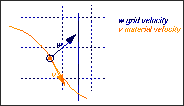
ALE stands for Arbitrary Lagrangian-Eulerian formulation. Material flows through an arbitrary moving mesh. Both the material and the mesh move with respect to the laboratory. It looks like a combination of Lagrangian and Eulerian formulations.
This formulation can be activated in RADIOSS for a specific part by a flag in the material data:
/ALE/MAT/mat_ID
Where, mat_ID is the identification number of the material to be set in ALE.
Grid velocities and displacements are arbitrary.
In practice, built-in algorithms determine smooth grid deformation according to displacements of the ALE domain boundaries. Several algorithms are available (DONEA, SPRINGS, DISP, and ZERO).
It is worthwhile to note that ALE formulation can be degenerated in Lagrangian (w=u: the grid velocity is equal to the material velocity) or in Eulerian (w=0: the grid velocity is set to zero).
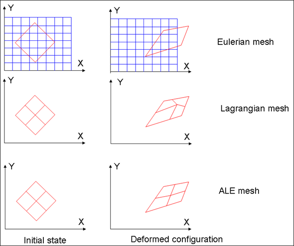
Eulerian, Lagrangian and ALE meshes
Boundary nodes between ALE and Lagrangian materials must be set to Lagrangian: grid and material velocities are equal. Boundary nodes between ALE and Eulerian materials must have their grid velocity set to zero.
Both conditions are set using the /ALE/BCS option: You can specify extended boundary conditions for ALE nodes (grid velocity components can be set to 0 or to the material velocity). The grid velocities can be imposed with ALE links to any nodes in a similar manner to classical kinematic conditions (option /VEL/ALE in Engine).
| Note: | When a solid element is connected to a shell element, the connected nodes are automatically set as Lagrangian. |
|
Nodal Boundary Conditions
By default, kinematic constraints act on material velocities and accelerations. In RADIOSS, you can define a wide variety of such constraints. For multi-physic and fluid applications, options are:
| • | fixed and full slip boundary conditions |
| • | imposed velocities (imposed flux at inlet) |
| • | rigid links (temporary adds during restarts) |
| • | rigid bodies to model rigid structures and connections and also to compute drag and lift forces (fluid impulse on rigid body is stored in time history database) |
Grid constraints act only on grid velocities. Specify:
| • | fixed and full slip grid conditions |
| • | Lagrangian conditions (grid and material velocity are equally set) |
| • | ALE links to maintain regular distribution of nodes |
| • | imposed grid velocities (moving inlet and outlet) |
Elementary Boundary Conditions
Boundary elements allow prescription of element values at domain boundaries. They can be specified by assigning material law 11 (or law 18 in Purely Thermal Material cases) to boundary elements (quads in 2D analysis and solids in 3D analysis) or EBCS to boundary faces of elements. For each variable P, rho, T, k, epsilon, internal energy, the following can be prescribed:
| • | imposed varying conditions according to user function |
| • | smoothly varying predefined function |
Non-reflective frontiers (NRF) (material 11, option 3) ensure free field impedance to pressure and velocity fields.
With RADIOSS ALE/CFD any combination of the above options can be specified; on the counterpart, the closure of the various convection and diffusion equations has to be verified carefully by you.
Generally the following elementary boundary conditions are used:
| • | Inlet, flux is imposed using imposed velocities; density, energy, turbulent energy (that is: k) are imposed as constants. Continuity is imposed for pressure (display purposes only) and for epsilon. Turbulent energy, rho k is set to zero for external flows and to 1.5*rho*(0.06 Vin)^2 for internal flows. |
| • | Outlet, continuity for all variables except pressure, which is imposed. When using the Non-reflective frontiers (NRF) option, you provide a value for sound speed and a typical relaxation length, which must be greater than the largest wave length of interest. |
| • | Sides, continuity for all variables with the Non-reflective frontiers (NRF) option or slip conditions without boundary elements. |
If an element does not exist at boundary, continuity is assumed; but kinematic conditions are necessary to disallow fluxes; otherwise the convection equation is not closed and the program can diverge.
Fluid/Structure Connection
At least one row of ALE elements should be used when fluid is in contact with shells.
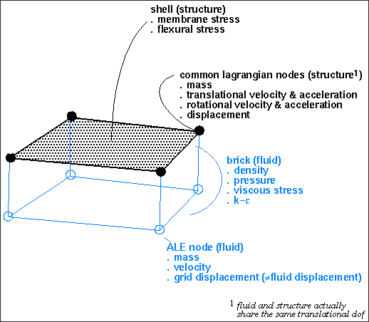
Example of mesh for fluid-structure interaction


