|
»Click here to display Table of Contents«
|

Methodology |

|

|

|

|
|
Methodology |
|
|
|

|
|
»Click here to display Table of Contents«
|
Methodology |
|
|
|
|
|
Methodology |
|
|
|
|
The purpose of this section is to show the several steps for the generation of a proper RADIOSS ALE/CFD model.
Usually, one receives a CAD model according to which the model should be build. The first task is to clean this CAD and perform simplifications:
| • | Add surfaces to close volumes used by automatic tetrahedral mesh |
| • | Add surface to control mesh progression |
| • | Patch surfaces to prepare mesh zones |
| o | Remove details whose size is smaller than what can be solved |
| o | Remove line constraints on surfaces whenever possible |
Only hexahedron elements (or quad elements in 2D analysis) are compatible with the ALE or Eulerian formulations. To create the mesh, the usual technique consists in meshing at first outer surfaces of each considered domain with triangles, then generating automatically an internal volume tetrahedron mesh and finally split the tetra's in four hexa each (watch closely the number of elements). Triangle mesh size should be 3.5 times larger than the planned mesh size for tetrahedral.
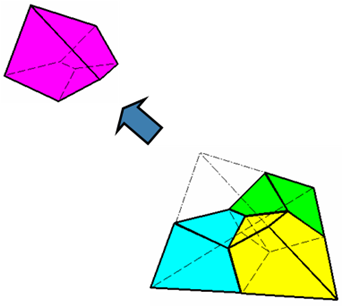
Tetrahedron transformed to hexahedron mesh
Some extrusions are added whenever necessary, for example:
| • | Outlet |
| • | Inlet |
| • | Non-reflective frontiers (NRF) |
| • | Tubes |
Of course, any other technique is suitable if generating hexahedron elements.
For boundary layers, the wall element size is determined as explained in Wall Element Size. The mesh for boundary layer is generally obtained by meshing the wall surface using triangles. Then, by extruding the surface mesh, a solid pentahedron mesh is created. The pentahedron elements can afterward be split easily to hexahedrons, as shown in the following figure.
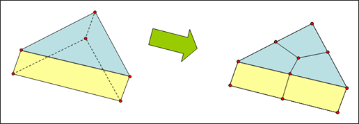
Split of a pentahedron element to three hexahedrons
Two aspects are involved when considering the mesh size:
| • | Velocity and pressure gradients: Near turbulent walls the mesh size is governed by the y+ value, which can range from 100 to 1000 or even higher (In pipes, y+ values as high as 8000 provide accurate results). From there, geometric progression is generally used toward coarser regions. |
| • | Acoustic accuracy: A maximum size can be derived from the minimum wave length of interest. Generally use of 12 elements per wave length is acceptable. |
Obviously the first condition will be governing region close to the obstacle or wall and the second will constrain the maximum size in the whole computational domain.
To build up a mesh, some trade-off is generally needed. The total time, Ttot, to be simulated can be evaluated as:
Ttot ~ 20 * L / c
L Largest model size
The total CPU needed, which is the major criterion to establish a trade-off between feasibility and accuracy can be estimated as:
CPU = Ttot/dtc * Number of element * cpu/el/cycle
The generation of the mesh in order to perform the desired simulation has to be carefully defined according to two criteria and a trade-off between feasibility (CPU time available) and precision:
| • | 10 elements minimum per vortex to be solved |
| • | Local Strouhal number not exceeding 1/6 for the frequency range of "interest" in regions of acoustic sources: |
Str = f h/v < 1/6
for example: fmax =600 Hz, v=30m/s => h ~ 8 mm
| • | Critical in region away from acoustic sources |
| • | Six elements per wave length along direction of propagation |
for example: fmax = 600 Hz, c=300 m/s => h ~ 8cm
Between the available CPU total time to be simulated and the critical time step; the time step will automatically be set to satisfy Courant's condition:
dt = Min (h) / c
Total time should be a multiple of the smallest frequency present in the model. Total CPU time is proportional to the number of cycles (final time divided by time step), the number of elements and the cost of each element (depends on the computer):
T = Ncycle * Nelem * Cost / cycle / elem
Practically, it is advised to perform a timing on a couple of cycles (do not forget to subtract the time of initialization) in order to know the cost per cycle of the simulation before launching a large simulation.
Consider the case of airflow passing over an obstacle is studied (Figure below) where the aim of the simulation is to measure the noise generated by this flow in any location of the mesh. The mesh should have at least four different regions (refer to Mesh Generation):
| • | Coarse mesh (all the computational domain except the immediate surroundings of the obstacle) |
| • | Refined mesh (close to the obstacle) |
| • | Inlet element (one row of elements) |
| • | Outlet elements (one row of elements) |
With l the characteristic size of the obstacle in the flow, there are typically three different mesh zones:
Zone |
Typical Size of Elements |
Note |
|---|---|---|
very fine |
a |
Chosen such as the obstacle is descretized with a minimum of 20 cells in each direction. |
fine |
2a to 3a |
|
course |
4a to 6a |
Make sure the course cells are appropriate for convection of the highest frequencies of interest. |
If the highest frequency of interest in the problem is f, then no cell in the mesh should be bigger than:
Size of element < C / 10.f
Where, C is the speed of sound in the fluid.
Inlet and outlet element thickness should be 1/10 of the neighboring elements of the computational domain.
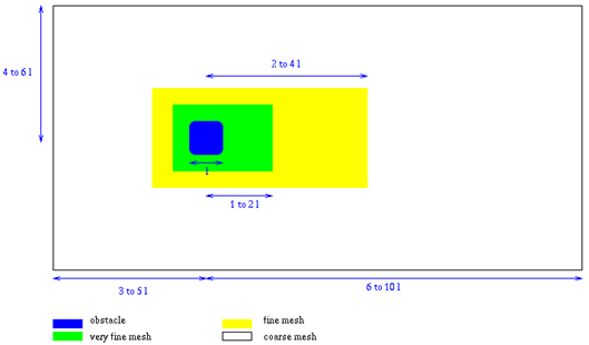
Number of elements for typical mesh for CAA problems (may vary for specific applications)
For problems with low Mach numbers (lower than 0.2), satisfactory results can be obtained under the quasi-compressibility assumption. This will save time on the computation. The compressibility implies that Navier-Stokes equations include wave equation. Then, acoustics and fluid flow can be treated at the same time, providing high numerical accuracy. Quasi-compressibility means, transport terms except in the momentum equation are neglected. Therefore, by reducing C1 in hydrodynamic material laws, the sound speed decreases and the time step increases (for example by dividing the C1 value by 10, the time step can be multiplied by 3).