A classification of Aero-Acoustic problems can be made using the following three categories:
| • | External wind noise transmitted to the inside through a structure: In the automotive industry, a pillar, side mirror and windshield wipers noise are typical problems of this category. |
| • | Internal flow noise transmitted to the outside through a structure: Examples of this type of problem are: exhaust, HVAC and intakes noises. |
| • | Rotating machines noise: Axial and centrifugal fans are noisy components that bring with them many interesting Aero-Acoustic problems. |
The purpose of this section is to show how to generate a proper ALE/CFD model for CAA applications. Consider the case of airflow passing over an obstacle. The purpose of the simulation is to measure the noise generated by this flow in any location of the mesh.
Output
The ability to post-process the noise generated by the flow will depend on the definition of output elements for time history recording. Those elements should be chosen at locations where noise is to be computed.
A series of elements and nodes in the system are saved in the time history file. The signals are recorded in each element and nodes and can be analyzed by FFT in order to determine a SPL map and evaluate the power level of the source.
It is also possible to save evolution with time of the different parts in the system and the rigid body.
RADIOSS CAA Methodology
The methodology for CAA simulation is as follows:
| • | Generate a RADIOSS model using a mesh generation and introduce RADIOSS specific options for analysis. |
| • | Run a first simulation with the model until a quasi-steady state is reached, from a uniform initial velocity field. This can be checked by looking at the model Kinetic Energy in the time history. |
| • | During a second simulation, record a time domain signal at the locations where the noise is to be analyzed. |
The two simulations can be combined into one. The main point is to make sure the time domain signal is not recorded before the steady state is reached for the whole model.
A couple of useful rules are listed below:
| • | Memory required to run the simulation (in words) ~ 100*Nelts + 6*Numnod*8*Nprocs used in parallel. |
| • | Time step is governed by sound speed and mesh size.
Where, c is the sound velocity (c=344m/s in the air) and u is the local flow speed. |
| • | Convergence depends on the case but should roughly be obtained after two to three periods of the lowest frequency considered. |
| • | Frequency resolution is 1/(recording time) of the @T file so recording time must be 1/Fmin |
| • | Sampling recording must be > 4.fmax |
| • | Approximately six elements per shortest wavelength must be present in the model. (l=c/f in the far field, u/f close to the sources). |
A constant time step is recommended. This can be activated by using the following command in the Engine deck:
/DT/SHELL/CST
(scale factor) (time step greater than the critical one)
Whenever shells are not present, this command is irrelevant and the following alternate command should be used:
/DTIX
(initial time step) (maximum time step)
In this case, you should provide a time step value smaller than the effective critical time step for both items initial and maximum time step.
High frequency cutoff is performed above Nyquist frequency to avoid frequency folding in the discrete Fourier transform. Numerical filtering is performed using coefficients of a classical linear phase filter.
Frequency resolution is the invert of physical time duration, no matter which sampling frequency you are using. For a frequency interval [fmin,fmax], the simulated time, T must be greater than 1/ fmin, the sampling frequency, fs must be greater than 4*fmax; RADIOSS will produce N=fs. T samples, T has to be chosen so that N=2n for subsequent Fast Fourier Transform.
10000 Hz is a typical sampling value for exhaust noise analysis.
Example of filter characteristics:
| • | number of coefficients: 1320 |
| • | base computational frequency fc = 1/dtc = 2.22 10^6 Hz (dtc, critical time step) |
| • | sampling frequency for output fs = 10040 Hz |
| • | Nyquist frequency or cut off fcut = 5020 Hz |
No attention or risk of folding is actually obtained in the 0-2500 Hz range.
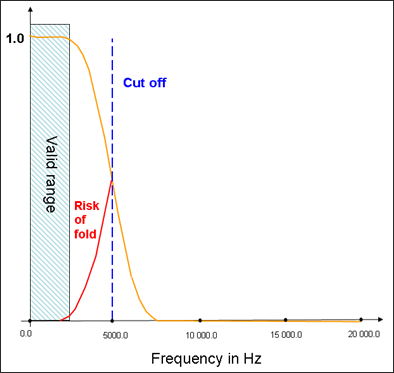
Example of filtering
Note that the sampling frequency is reset so fc/fs is an integer.
ALE Subcycling (/ALESUB)
As the critical time step is higher for a gas than for a solid, different time steps can be used in ALE and Lagrangian parts. This allows you to increase the performance.
The option /ALESUB can be activated in RADIOSS Engine deck as follows:
/ALESUB
 1.
1.
Where, is the scale factor on time step for ALE elements, which must be less than or equal to 1.


