The Smooth Particle Hydrodynamics method formulation is used to solve the equations of mechanics, when particles are free from a meshing grid. It is specially adapted to simulate phenomena with a very substantial deformation, that is a range of applications where the Finite Element method, with ALE and Lagrangian formulation, loses' its efficiency and accuracy.
The SPH method built in the RADIOSS code is compatible with most functions. For instance, it is possible to cause two objects to interact, one discretized by finite elements and the other by particles.
You can put the SPH formulation in an ALE model, only if the boundary between SPH and ALE is Lagrangian. The SPH formulation is only available in 3D analysis.
SPH Cells Distribution
The particles should be distributed through a hexagonal compact or a cubic net.
Hexagonal Compact Net
A cubic centered faces net realizes a hexagonal compact distribution, which can be useful to build the net.
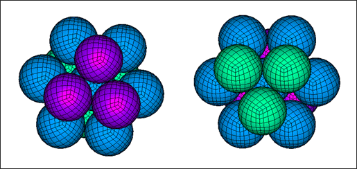
Local views of the hexagonal compact net
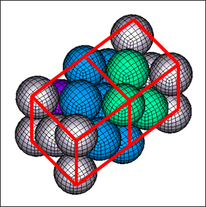
Perspective view of the cubic centered faces net
The nominal value h0 of h for the hexagonal compact net is the distance between any particle and its closest neighbor.
The mass of the particle which will be considered is the mass mp defined in the property which is associated to the part that the particle belongs to.
The mass of the particles mp should relate to the density of the material  and to the size h0 of the hexagonal compact net, with respect to the following equation:

Since the space can be partitioned into polyhedras surrounding each particle of the net, each one with a volume:

Notice that choosing h0 for the smoothing length insures naturally consistency up to order one, if the previous equation is satisfied.
Weight functions vanish at distance 2h where, h is the smoothing length. In a hexagonal compact net with size h0, each particle has exactly 54 neighbors within the distance 2h0:
Number of Neighbors in a Hexagonal Compact Net
Distance d
|
Number of particles
at distance d
|
Number of particles
within distance d
|
h0
|
12
|
12
|
|
6
|
18
|
|
24
|
42
|
2h0
|
12
|
54
|
|
24
|
78
|
If SPH correction is used, notice that a small value for the smoothing length will increase the instability of the SPH method in case of tension behavior.
So, if using a hexagonal compact net and SPH corrections, it is recommended to set the smoothing length lower than the inter-particles minimum distance, only when there is no tension in the physical problem.
In the case of tension behavior, the value of the smoothing length can be set somewhat larger than the inter-particles distance, in order to limit the tension instability of SPH method. But a large value will result in excessive computational time.
Cubic Net
Let, c the side length of each elementary cube into the net.
The mass of the particles mp should relate to the density of the material  and to the size c of the net, with respect to the following equation:

Number of Neighbors in a Cubic Net
Distance d
|
Number of particles
at distance d
|
Number of particles
within distance d
|
c
|
6
|
6
|
|
12
|
18
|
|
8
|
26
|
2c
|
6
|
32
|
|
24
|
56
|
|
24
|
80
|
|
12
|
92
|
3c
|
6
|
98
|
From experience, a larger number of neighbors should be taken into account than in the hexagonal compact net, in order to solve the tension instability. A value of the smoothing length between 1.25c and 1.5c seems to be well-suited.
If choosing the smoothing length h=1.5c, each particle has 98 neighbors within the distance 2h.
Maximum Number of Neighbors to be Stored
When more than Nneigh neighbors are found within the security distance, the program retains the only Nneigh closest points and decreases the value of asort.
If when doing this, all true neighbors lying inside the influence sphere of all particles are still retained, then the results do not change.
In the other case, a message such as "Warning SPH Computation" is sent to the RADIOSS output file. Note that in the case of such a message, the computation time increases since it becomes necessary to sort closest particles at each cycle. Moreover, this kind of situation has to be analyzed carefully since it is often put into an evidence (local) instability.
SPH Symmetry Conditions
Use of Multiple SPH Symmetry Conditions
An axi-symmetry condition can be modelized through the use of two conditions with respect to two planes intersecting at the axis of symmetry. A spheric symmetry condition can be modelized through the use of three conditions with respect to three planes intersecting at the center of symmetry.
Nevertheless, these kinds of symmetries are not treated the same way.
For instance, in case of an axi-symmetry condition, not all ghost particles are built around the axis of symmetry. The only symmetric particles of real particles with respect to the two symmetry planes are built.
Multiple symmetries are not complete
Therefore, some characteristics of axi-symmetry (respectively spheric symmetry) conditions can be closed to the axis of symmetry (respectively the center of symmetry).
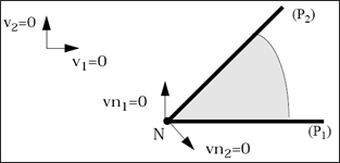
Nodes closed to the axis of symmetry (resp. the center of symmetry) and lying on a symmetry plane (P) can get a normal to (P) velocity which is non-zero, since their neighborhood is not symmetric with respect to plane (P).
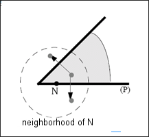
Neighborhood of particle N is not symmetric with respect to plane (P) and N’s normal velocity to plane (P) can be non-zero
A Kinematic Boundary Condition
With respect to the previous discussion: adding the kinematic boundary condition an explicit way allows to enforce it.
A kinematic boundary condition will be added to the nodes belonging to the nodes group specified into the /SPHBCS option, so that:
| • | if type is "Slide", the velocity of the node in direction "Dir" is set to zero |
| • | if type is "Tied", the velocity of the node in all directions is set to zero |
In case of several kinematic boundary conditions applied to the same node through different SPH symmetry conditions, the kinematic boundary conditions are composed automatically, even if the kinematic boundary conditions are applied into non-orthogonal directions.
Combination of kinematic boundary conditions from different SPH symmetry conditions
The figure above indicates that if two kinematic boundary conditions are applied to N through two symmetry conditions with respect to planes (P1) and (P2), the two boundary conditions are modified so that the velocity in the plane normal to common axis of (P1) and (P2) will remain zero. Note that if one of the two symmetry conditions is a type "Tied" condition, the velocity of N in all directions is set to zero.
It also allows application to the same node, a kinematic boundary condition through a SPH symmetry condition (option /SPHBCS) and a standard boundary condition (option /BCS) at the same time, as long as the standard boundary condition is not given in a moving skew system, but a fix skew system or the global skew system. The two conditions are then composed the same way.
Part Mass
You must be advised that when a particle lies on a symmetry plane at time t=0, the mass and the initial volume considered for the particles are respectively:
Where, mp is the mass specified into property set.
When a particle lies on n symmetry planes at time t=0,
Ghost particles built from this particle will get the same initial volume and mass.
When n > 2, the previous equation may provide an error on mass and energies output for the part the particles belong to, with respect to the physical model.
Formulation Level
When a symmetry plane is defined, and even if a kinematic condition is set for all particles lying on the symmetry plane, particles lying at time zero inside the domain are theoretically able to cross the symmetry plane.
This is specific to SPH for which stiffness between particles does not increase to an infinite value when particles collapse. So it can occur when the particles, which lie on the symmetry plane let the particles which were inside the domain go through the symmetry plane.
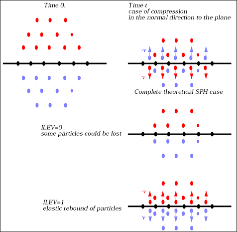
Formulation level
If Ilev =0, particles crossing the symmetry plane will be (progressively) not taken into account anymore in the computation, neither than their symmetric particles which then lie inside the domain.
If Ilev =1, particles which have crossed the symmetry plane rebound an elastic way upon the symmetry plane: their velocity in the normal direction to the plane is set the opposite.
Note that when Ilev =1, it is strongly recommended to associate kinematic condition to all particles lying on symmetry plane at time zero, for computational time reasons.
Maximum Number of Ghost Particles Created
Ghost particles are created at each search for neighbors time within the security distance, and then destroyed when a new search occurs (a new set of ghost particles is then created).
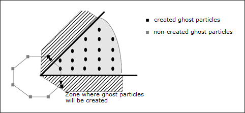
At any search time, all ghost particles which are inside the security distance of any real particle are created.
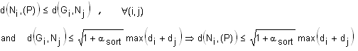
In practice, some more particles, strictly necessary, are created: a symmetric particle Gi to particle Ni is created, with respect to symmetry plane P, if:
 neighbor of
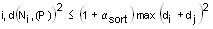
As long as no real particles cross the symmetry plane (all real particles lie on the same side of the symmetry plane), this criteria is sufficient to get all ghost neighbors of all real particles inside the security distance, since:
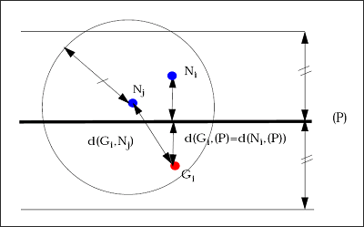
Ghost particles to be created
Particles, which one can expect to remain far from the symmetry plane all along the simulation, will never be symmetrized. This gives a way to over-estimate the number of particles which will be symmetrized at one time.
When a particle Ni has to be symmetrized with respect to n conditions, the particle Ni gives birth to n ghost particles. The following quantity must remain less than "Nghost".
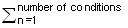 | number of particles to be symmetrized with respect to condition n |
Anyway, the default value which is the number of SPH symmetry conditions multiplied by the number of particles will be enough to treat any problem.
Solid to SPH options (Sol2SPH)
The solid to SPH option (Sol2SPH) enables you to turn a solid element into particles either in order to increase the time step/robustness of a Lagrangian calculation, while not changing the physics.


