OS-1500: Nonlinear Implicit Analysis of Bending of a Plate

The purpose of this tutorial is to demonstrate how to carry out nonlinear implicit analysis in OptiStruct by simulating the bending of a plate under constant pressure.

Model Description

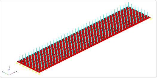
The figure below illustrates the structural model used for this tutorial: a long rectangular plate which is supported at one end and distributed load is applied on the top surface. The dimensions of the plate and material parameters can be obtained in the table below.

rd2090_plate_model

Units	Length: mm; Time: s; Mass: Mgg; (Force: N; Stress: MPa)
Length	1000 mm
Width	200 mm
Thickness	4.0 mm
Material	Steel, Elasto-plastic, using Johnson-Cook law
	Initial density ():	7.90e-9 kg/mm3
	Young's modulus (E):	200000 MPa
	Poisson coefficient (ν):	0.29
	Yield Stress (0):	100.0 MPa
	Hardening Parameter (b):	1.0MPa
Imposed pressure	0.02 MPa, applied normal to the plate
Simulation time	[0 – 1.0 s]

The following exercises are included in this tutorial:

•	Create plastic material and corresponding shell property

•	Set up boundary conditions and imposed velocity

•	Set up implicit analysis

•	Submit job and view result

Exercise

Step 1: Import the model

1.	Launch HyperMesh Desktop. The User Profiles dialog appears.

2.	Select OptiStruct and click OK. This loads the user profile.

3.	Click File > Import > Solver Deck.

4.	For the File type:, select OptiStruct.

5.	Select the Files icon . A Select OptiStruct File browser opens.

6.	Select the plate.fem file you saved to your working directory from the optistruct.zip file. Refer to Accessing the Model Files.

7.	Click Open > Import.

8.	The plate.fem OptiStruct input file is loaded into the current HyperMesh session.

9.	Click Close to exit the tab.

Step 2: Define Unit System

1.	From the Analysis page, select control cards.

2.	Select DTI_UNITS, and set parameters, as shown below.

rd2090_dti_units

3.	Click return twice to go to the main menu.

Step 3: Update the Material

1.	In the Model browser, click on the material MAT1_1.

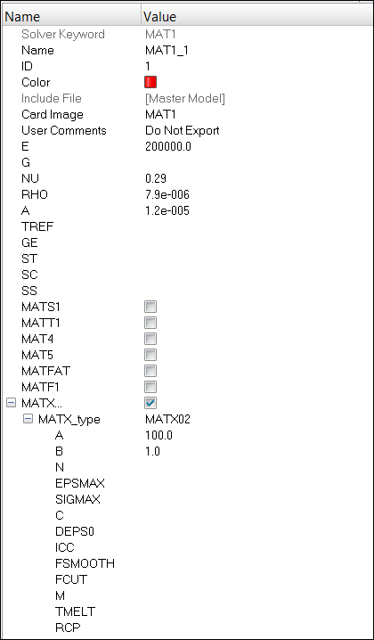
2.	Check the box next to MATX and select MATX02 for the MATX_type field to define additional material properties for Johnson-Cooke elastic-plastic material for geometric non-linear analysis.

3.	Input the values as shown below. See material parameters for details.

OS_1500_01

Step 4: Update the Property

1.	In the Model browser, click on the property PSHELL_1.

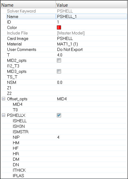
2.	Check the box next to PSHELLX (to define additional SHELL properties for geometric non-linear analysis).

3.	Input the values as shown below. See shell parameters for details.

OS_1500_02

Step 5: Create Boundary Condition

1.	In the Model browser, right-click and select Create > Load Collector.

2.	For Name, enter LC_SPC.

3.	Click Color and select a color from the color palette.

4.	For Card Image, select None from the drop-down menu.

5.	From the Analysis page, select constraints, toggle create.

6.	Switch entity selector to nodes and select the nodes shown below.

rd2090_nodes

7.	Select the degrees of freedom dof1 and dof3. Deselect all others.

8.	For load types, select SPC.

9.	Click create to create the boundary constraints.

10.	Next, select the bottom two nodes, as shown below.

rd2090_nodes_2

11.	Select the degrees of freedom dof1, dof2 and dof3. Deselect all others.

12.	For load types, select SPC.

13.	Click create to create the boundary constraints.

14.	Click return to go to the main menu.

Step 6: Create Imposed Load

1.	In the Model browser, right-click and select Create > Load Collector.

2.	For Name, enter LC_PLOAD.

3.	Click Color and select a color from the color palette.

4.	For Card Image, select None from the drop-down menu.

5.	From the Analysis page, click pressures and toggle create.

6.	Switch entity selector to elems and select all elements.

7.	Click on the toggle next to magnitude= and switch pressure definition method to constant vector.

8.	For magnitude, enter -0.02.

9.	For load types, make sure to select PLOAD as the load type.

10.	Click create > return.

11.	Create a load collector (using steps 6.1 to 6.3) named TH_IMPLOAD, with Card Image set to TABLED1.

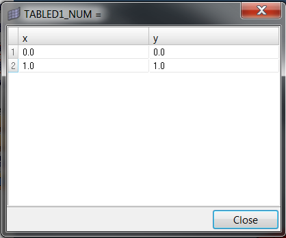
12.	For TABLED1_NUM, enter 2 and press enter.

13.	Click the Table icon next to Data and enter the values shown below in the pop-out window.

OS_1500_03

14.	Click Close. A curve is now created.

15.	Create a new load collector named LC_IMPLOAD with Card Image set to NLOAD1.

16.	For EXCITEID, click Unspecified > Loadcol.

17.	In the Select Loadcol dialog, select LC_PLOAD.

18.	For TID, click Unspecified > Loadcol.

19.	In the Select Loadcol dialog, select TH_IMPLOAD.

Step 7: Define implicit analysis parameters

1.	In the Model browser, right-click and select Create > Load Collector.

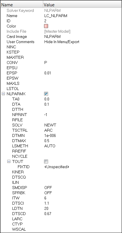
2.	For Name, enter LC_NLPARM.

3.	For Card Image, select NLPARM.

4.	Select the CONV as P with a EPSP of 0.01.

5.	Check the box next to NLPARMX. This defines the parameters for implicit nonlinear analysis iteration strategy.

6.	Input the values as shown below. See nonlinear analysis control parameters for details.

OS_1500_04

Step 8: Define Output Control parameters

1.	From the Analysis page, select control cards.

2.	Click on GLOBAL_OUTPUT_REQUEST.

3.	For DISPLACEMENT, ELFORCE, OLOAD, STRESS, and STRAIN, set Option to Yes.

4.	Click return twice to go to the main menu.

Step 9: Create implicit analysis subcase (also referred to as a loadstep)

1.	In the Model browser, right-click and select Create > Load Step.

2.	For Name, enter sub_nlgeom_implicit.

3.	For Analysis type, select geometric non-linear from the drop-down menu.

4.	For SPC, click Unspecified > Loadcol.

5.	In the Select Loadcol dialog, select LC_SPC from the list of load collectors and click OK.

6.	For NLOAD, click Unspecified > Loadcol.

7.	In the Select Loadcol dialog, select LC_IMPLOAD from the list of load collectors and click OK.

8.	For NLPARM, click Unspecified > Loadcol.

9.	In the Select Loadcol dialog, select LC_NLPARM from the list of load collectors and click OK.

10.	For TTERM, enter a value of 1.0.

Step 10: Submit the job

1.	From the Analysis page, select OptiStruct.

2.	Click save as and select the directory where you want to write the file.

3.	For File Name, enter plate.fem and click Save. The file extension .fem is necessary for OptiStruct to recognize it as an input file.

4.	Set the export options toggle to all.

5.	Set the run options toggle to analysis.

6.	Set the memory options toggle to memory default.

7.	Click OptiStruct. This launches the OptiStruct job.

If the job is successful, the new results files is located in the directory where HyperMesh was invoked. The plate.out file is where you will find error messages that will help you debug your input deck, if any errors are present.

The default files that will be written to your directory are:

plate.html	HTML report of the analysis, giving a summary of the problem formulation and the analysis results.
plate.out	ASCII based output file of the model check run before the simulation begins and gives some basic information on the results of the run.
plate.stat	Summary of analysis process, providing CPU information for each step during the process.
plate.h3d	HyperView compressed binary results file.

Step 11: View analysis results

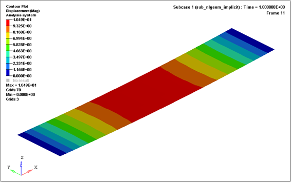
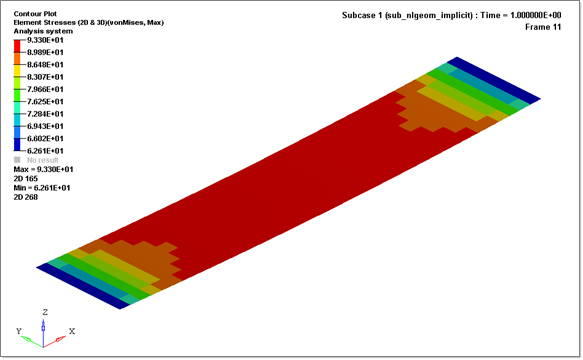
1.	Using HyperView, plot the Displacement and the von Mises stress contour at 1.0 s.

rd2090_contour_plot

rd2090_contour_plot_2