In this tutorial, an existing finite element model of an aluminum wing rib model is used to demonstrate how to perform nonlinear gap analysis using OptiStruct. HyperView is used to post-process the stress and deformation characteristics of the rib.

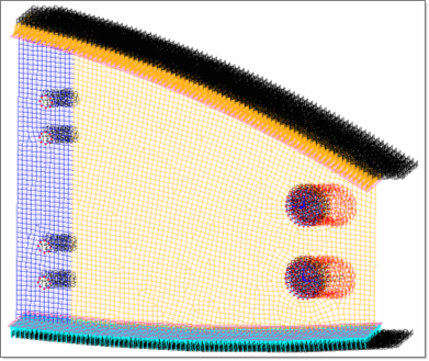
Wing rib model
There are four shell components in the model: the mounting flange, the web, the top and bottom flanges, and the lug. Gap elements have already been defined in the model and they connect the web to the lug. Coupling forces are applied to the lug and pressure loading has been defined on the top and bottom flanges of the rib joint. The mounting flange is constrained in all degrees of freedom at the four mounting hole locations and the lug is constrained for the z-displacements and rotations to prevent rigid body motion.
The following exercises are included:
Exercise 1: Linear gap analysis on the aircraft rib
| • | Create a cylindrical coordinate system and assign it to the gap elements |
| • | Create a gap property and assign it to the gap elements |
| • | Run a linear gap analysis |
| • | Post-process the results from the linear gap analysis using HyperView |
Exercise 2: Nonlinear gap analysis on the aircraft rib
| • | Create a load collector to define nonlinear parameters |
| • | Update the subcases to include the nonlinear load collectors |
| • | Run a nonlinear gap static analysis |
| • | Post-process results using HyperView |
Exercise 1: Linear Gap Analysis
Step 1: Load the User Profile and Retrieve the Model File
| 2. | Select OptiStruct in the User Profiles dialog. This loads the user profile. It includes the appropriate template, macro menu, and import reader, paring down the functionality of HyperMesh to what is relevant for generating models for OptiStruct. |
| 3. | Click File > Open. An Open Model browser window opens. |
| Note: | If HyperMesh Desktop was launched, use: File > Open > Model. |
|
| 4. | Select the rib.hm file you saved to your working directory from the optistruct.zip file. Refer to Accessing the Model Files. |
| 5. | Click Open. The rib.hm database is loaded into the current HyperMesh session, replacing any existing data. The database only contains geometric data. |
The location of rib.hm displays in the file: field.
Step 2: Create a cylindrical coordinate system and assign it to the gap elements
For gap elements with coincident nodes as is the case here, the gap coordinate system MUST be specified. For detailed information, refer to the Help section on CGAP.
| 1. | In the Model browser, right-click and select Create > System Collector. |
| 2. | For Name, enter cylindrical. |
| 3. | Click Color and select a color from the color palette. |
| 4. | In the Model tab, hide all load collectors by right-clicking on Load Collector > Hide. |
| 5. | In the Model browser, click the Isolate Shown icon  . . |
| 6. | Expand the Component list and select the Lug component. This isolates the display of only the Lug component. |
| 7. | Click the XY Top Plane View icon  to set the model view. to set the model view. |
| 8. | Click Geometry > Create > Systems > Axis Direction to open the Systems panel. |
| 9. | The cyan halo around the yellow nodes button indicates that it is the current option. Select the center node on the upper lug. |
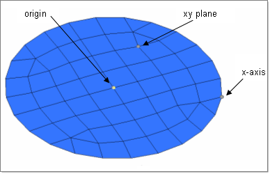
| 10. | Click origin and select the center node again, click x-axis, select any node on the circumference and for xy plane, select any node on the plane of the lug, as shown in the following figure: |

Nodes to select for creating cylindrical coordinate system
| 11. | Click the switch beside rectangular and select cylindrical. |
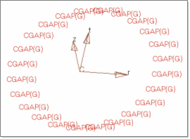
For cylindrical systems, the x-axis defines the radial direction (q= 0) and the xy plane defines the r-q plane.
| 13. | Repeat this process for the bottom lug (steps 9 through 12 of this sequence). |
| 15. | Click the Model tab to activate the Model browser, if you left it. |
| 16. | Select only the gap component. With Isolate Shown still active this displays only the gap component. |
| 17. | Click the Card Editor icon  . . |
| 18. | Click the entity selection switch on the top left of this panel and select elems. |
| 19. | Click elems >> by window from the pop-up menu. |
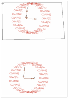
| 20. | Select the gap elements that are connected to the top lug, as shown by the selected window in the following figure. |

Gap elements connected to top lug
| 21. | Click select entities. |
| 22. | Click config= and select gap from the pop-up menu. |
| 24. | Click CID, and select the system that was created at the center of the top lug, as shown below. |

| 25. | Click return twice to go back to the main menu. |
| 26. | Repeat this process for the gap elements that are connected to the bottom lug. The gap elements have now been assigned with a cylindrical coordinate system. |
Step 3: Define a property card and assign it to the gap elements
| 1. | In the Model browser, right-click and select Create > Property. |
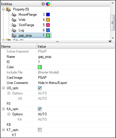
| 2. | For Name, enter gap_prop. |
| 3. | Click Color and select a color from the color palette. |
| 4. | For Card Image, select PGAP and click Yes to confirm. |
| 5. | Make sure the check box next to U0_opts is checked. This way the initial gap opening is calculated automatically. |
| 6. | Make sure the check box next to KA_opts is checked. This determines the value of KA for each gap element using the stiffness of surrounding elements automatically. |

| 7. | Click Mesh > Create > 1D Elements > Gaps to open the Gaps panel. |
| 8. | Select the update subpanel. |
| 9. | Click elems >> by collector. |
| 10. | Select gap by checking the box beside it. |
| 11. | Click the green select button. |
| 12. | Click property= and click on gap_prop. |
| 14. | Check beside property. |
| 15. | Click update. The gap elements have now been updated to the new property collector. |
Step 4: Run a linear gap analysis
Two loadsteps have already been created in this HyperMesh model.
| 1. | From the Analysis page, click OptiStruct. |
| 2. | Click save as following the input file: field. A Save As browser window opens. |
| 3. | Select the directory where you would like to write the file and enter the name rib_linear.fem in the File name: field. |
The name and location of the rib_linear.fem file displays in the input file: field.
| 5. | Set the export options: toggle to all. |
| 6. | Set the run options: toggle to analysis. |
| 7. | Set the memory options: toggle to memory default. |
| 8. | Click OptiStruct. This launches the OptiStruct job. |
If the job was successful, new results files can be seen in the directory where the OptiStruct model file rib_linear.fem was written. The rib_linear.out file is a good place to look for error messages that will help to debug the input deck if any errors are present.
The default files written to the directory are:
rib_linear.html
|
HTML report of the analysis, giving a summary of the problem formulation and the results.
|
rib_linear.out
|
OptiStruct output file containing specific information on the file setup, the setup of the problem, estimates for the amount of RAM and disk space required for the run and compute time information. Review this file for warnings and errors that are flagged from processing the rib_linear.fem file.
|
rib_linear.h3d
|
HyperView binary results file.
|
rib_linear.res
|
HyperMesh binary results file.
|
rib_linear.stat
|
Summary of analysis process, providing CPU information for each step during analysis process.
|
Step 5: Post-process the results using HyperView
| 1. | From the OptiStruct panel, click HyperView. This will launch HyperView and load the rib_linear.mvw file, reading the model and results. |
| 2. | Click the Curves Attributes icon  and hide all components except the Web component. You can do this by activating the Auto apply mode: check box, (activating Display Off) and then clicking on the components that you want turned off in the Graphic User Interface (GUI). and hide all components except the Web component. You can do this by activating the Auto apply mode: check box, (activating Display Off) and then clicking on the components that you want turned off in the Graphic User Interface (GUI). |

| 3. | Go to the Contour  panel. panel. |
| 4. | Select the first pull-down menu below Result type: and select Element Stresses (2D & 3D). |
| 5. | Select the second pull-down menu below Result type: and select vonMises. |
| 6. | Above the Results browser in the left hand panel are the Load Case and Simulation Selection drop-down menus. |

| 7. | Select Subcase 1 (Coup_Vert) from the Load Case drop-down menu. |
| 8. | Click the XY Top Plane View icon  to display a top view of the Web. to display a top view of the Web. |
| 9. | Click Apply. This should show the contour of stresses on the Web component under the coupled loading. |

Stress results on the Web from linear gap analysis
| 10. | Click Delete Page  to end the HyperView session. to end the HyperView session. |
Exercise 2: Nonlinear Gap Analysis
Step 1: Create a load collector defining parameters for nonlinear static analysis
| 1. | In the Model browser, right-click and select Create > Load Collector. |
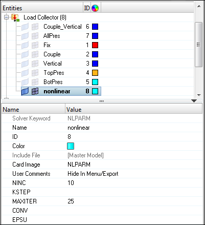
| 2. | For Name, enter nonlinear. |
| 3. | Click Color and select a color from the color palette. |
| 4. | For Card Image, select NLPARM from the menu. |
| 5. | Click NINC and enter 10. |
NINC denotes the number of load sub-increments. If NINC is blank, then the entire loading is applied at once. An NINC of 10 signifies that the load will be sub-divided into 10 equal increments.
| 6. | Click MAXITER and leave the default value of 25. |
| 7. | The error tolerances EPSU, EPSP and EPSW can be left at their default values. |
For details on these tolerances, read the section Nonlinear Quasi-static Gap and Contact Analysis in the online help.

Step 2: Update the loadsteps to include the nonlinear step
| 1. | Open the Load Step folder in the Model browser. |
| 2. | Click the Coup_Vert load step to open the Entity Editor. |
| 3. | For NLPARM, click Unspecified > Loadcol. |
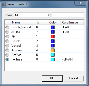
| 4. | In the Select Loadcol dialog, select the nonlinear load collector and click OK. |

| 5. | Repeat this process for the Pressure load step. |
Step 3: Run a nonlinear gap analysis
| 1. | From the Analysis page, enter the OptiStruct panel. |
| 2. | Click save as following the input file: field. A Save As browser window opens. |
| 3. | Select the directory where you would like to write the file and enter the name for the rib_nonlinear.fem, in the File name: field. |
The name and location of the rib_nonlinear.fem file displays in the input file: field.
| 5. | Set the export options: toggle to all. |
| 6. | Set the run options: toggle to analysis. |
| 7. | Set the memory options: toggle to memory default. |
| 8. | Click OptiStruct. This launches the OptiStruct job. |
If the job was successful, new results files can be seen in the directory where the OptiStruct model file rib_nonlinear.fem was written. The rib_nonlinear.out file is a good place to look for error messages that will help to debug the input deck, if any errors are present.
The default files written to the directory are:
rib_nonlinear.html
|
HTML report of the analysis, giving a summary of the problem formulation and the results.
|
rib_nonlinear.out
|
OptiStruct output file containing specific information on the file setup, the setup of the problem, estimates for the amount of RAM and disk space required for the run and compute time information. Review this file for warnings and errors that are flagged from processing the rib_nonlinear.fem file.
|
rib_nonlinear.res
|
HyperMesh binary results file.
|
rib_nonlinear.h3d
|
HyperView binary results file.
|
rib_nonlinear.stat
|
Summary of analysis process, providing CPU information for each step during analysis process.
|
Step 4: Post-process results using HyperView
| 1. | From the OptiStruct panel, click HyperView. This will launch HyperView and load the rib_nonlinear.h3d file, reading the model and results. |
| 2. | Go to the Curves attributes panel  and hide all the components except the Web component. You can do that by activating the Auto apply mode: to Display Off and then clicking the components that you want turned off in the GUI. and hide all the components except the Web component. You can do that by activating the Auto apply mode: to Display Off and then clicking the components that you want turned off in the GUI. |

| 3. | Click the Contour panel toolbar icon  . . |
| 4. | Select the first pull-down menu below Result type: and select Element Stresses (2D & 3D). |
| 5. | Select the second pull-down menu below Result type: and select vonMises. |
| 6. | Above the Results browser in the left hand panel are the Load Case and Simulation Selection drop-down menus. |
| 7. | Click Load Case > Subcase 1 (Coup_Vert). |
| 8. | Click the XY Top Plane View icon  to display a top view of the Web. to display a top view of the Web. |
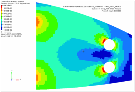
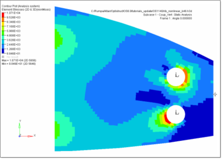
| 9. | Click Apply. This should show the contour of stresses on the Web component under the coupled loading. |

Stress results on the Web from nonlinear gap analysis.
Analysis Review
Even though the deformation patterns are similar for both linear and nonlinear analyses, the stress patterns differ. Though the horizontal loads are in opposing directions in the lug, the stress distribution in the web for the linear run are the same around both the lug holes which is not correct. This happens as all the gaps are in a closed condition for the linear analysis. Nonlinear gap analysis gives more accurate representation. The gap status, open or closed, depending on loading condition can also be observed from the .out file (shown below):
ITERATION 0
NONLINEAR ITERATION SUMMARY Subcase 1
LOAD FACTOR: 0.1000
------------------------------------------------------------
Nonlinear Error Measures Gap Elem Status
ITER EUI EPI EWI Open Closed
------------------------------------------------------------
1 9.9000E+01 1.1659E+00 1.1659E+00 23 25
2 2.9097E-02 2.5218E+02 1.1274E+01 23 25
3 8.4208E-05 1.9063E+01 1.9427E-02 22 26
4 1.4632E-06 0.0000E+00 0.0000E+00 22 26
See Also:
OptiStruct Tutorials


