This tutorial demonstrates how to set up the random response analysis for the existing frequency response analysis model. The setup for frequency response analysis is that the flat plate has two loading conditions that will be subjected to a frequency-varying load excitation using the direct method.
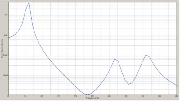
The PSD (power spectral density) for displacement at node 19 is output in the .rand file, and the peak values of PSD and RMS (root mean square) results are output to a .peak file. PSD and RMS stress results are output to a .op2 file and post-processed in HyperView.
The following exercises are included:
| • | Set up the problem in HyperMesh |
| • | Submit the OptiStruct job from within HyperMesh |
| • | View the results in HyperView |
Exercise
Setting up the Problem in HyperMesh
Step 1: Launch HyperMesh, set the OptiStruct User Profile and retrieve the structural model
| 2. | Select OptiStruct in the User Profiles dialog. |
| 3. | Click OK. This loads the user profile. It includes the appropriate template, macro menu, and import reader, paring down the functionality of HyperMesh to what is relevant for generating models for OptiStruct. |
| 4. | Click File > Open. An Open Model browser window opens. |
| Note: | If HyperMesh Desktop was launched, use: File > Open > Model. |
|
| 5. | Select the direct_psd.hm file you saved to your working directory from the optistruct.zip file. Refer to Accessing the Model Files. |
| 6. | Click Open. The direct_psd.hm database is loaded into the current HyperMesh session, replacing any existing data. The database only contains model data. |

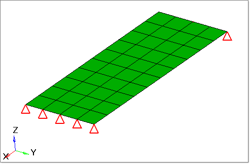
The frequency analysis setup is already made for this model where the one end of plate is clamped and the loading is applied on the other end (two different sources of the loading, thus two subcases). The loading frequency is defined by the FREQ1 card; from 20 to 1000 Hz with an interval of 20. The same loading frequency is applied on both the subcases.
Step 2: Create Load Collectors RANDPS and TABRND1
In this step, two PSDF of individual subcases and one coupled PSDF (meaning that those two subcases are correlated) are defined through RANDPS bulk data entry. RANDPS points to the table entity, TABRNDi.
| 1. | In the Model browser, right-click and select Create > Load Collector. |
| 2. | For Name, enter tabrnd1. |
| 3. | For Card Image, select TABRND1 from the drop-down menu. |
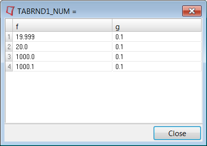
| 4. | For TABRND1_NUM, enter a value of 4 and press enter. |
| 5. | Input the parameters, as shown in the following image. |

| 7. | Create another load collector named randps. |
| 8. | For Card Image, select RANDPS. |
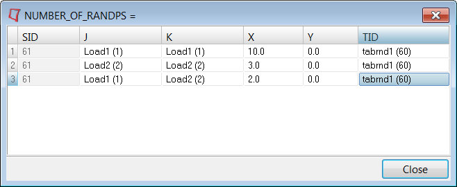
| 9. | Three RANDPS entries need to be defined. Input the values, as shown in the following image. The TABRND1 load collector is selected for the TID(i) column entries. |

Step 3: Add the RANDOM subcase information entry and output request
The RANDOM subcase information entry needs to be added to the frequency analysis model and the output commands for RMS and PSD results will be added as well.
| 1. | From the Analysis page, click control cards. |
| 2. | Go to GLOBAL_CASE_CONTROL panel. |
| 3. | Check the box in front of RANDOM and double-click the highlighted ID button and select randps. |
| 4. | Return to Control Cards and click GLOBAL_OUTPUT_REQUEST. Check the box for STRESS to activate the card edit panel. |
| 5. | Select OUTPUT2 as the FORMAT, PSDF under RANDOM, and YES under OPTION. RMS and PSDF stress are output to a .op2 file. |
| 6. | Click return to go back to the Control Cards panel. |
| 7. | Select CASE_UNSUPPORTED_CARDS and add the following cards: |
XYPLOT,DISP,PSDF/ 19(T3)
OptiStruct will output the PSDF for the translational displacement in z direction at node 19.
| 8. | Click OK, and then click return. |
Step 4: Submit the job
| 1. | From the Analysis page, click OptiStruct. |
| 2. | Click Save as following the input file: field. A Save As browser window opens. |
| 3. | Select the directory where you would like to write the file and enter the name for the direct_psd.fem in the File name: field. |
The name and location of the file displays in the input file: field.
| 5. | Set the export options: toggle to all. |
| 6. | Set the run options: toggle to Analysis. |
| 7. | Set the memory options: toggle to memory default. |
| 8. | Click OptiStruct. This launches the OptiStruct job. |
If the job completed successfully, new results files can be seen in the directory where the OptiStruct model file was written. The direct_psd.out file is a good place to look for error messages that will help to debug the input deck if any errors are present.
The default files written to the directory are:
direct_psd.html
|
HTML report of the analysis, giving a summary of the problem formulation and the results.
|
direct_psd.out
|
OptiStruct output file containing specific information on the file set up, the set up of the problem, estimate for the amount of RAM and disk space required for the run and compute time information. Review this file for warnings and errors that are flagged from processing the direct_psd.fem file.
|
direct_psd.h3d
|
HyperView binary results file.
|
direct_psd.stat
|
Summary of analysis process, providing CPU information for each step during analysis process.
|
Also, the following files will be output and which are specific to the random response analysis.
direct_psd.peak
|
ASCII result file, containing RMS and peak values of PSD.
|
direct_psd.rand
|
ASCII result file, containing PSD results.
|
direct_psd_rand.mvw
|
HyperView script file. This file will automatically create the plot of PSD over the frequency for the results contained in .rand file.
|
direct_psd.op2
|
Binary file containing RMS and PSD results.
|
Step 5: View the RMS and PSD results
This step describes how to post-process the RMS and PSD results in HyperView. The PSD for displacement at node 19 is output to direct_psd.rand file and the plot of PSD vs. frequency can be viewed by loading the direct_psd_rand.mvw file. The RMS and PSD stress results are available in .op2 file. The RMS and the peak values of PSD for displacement at node 19 are output to .peak file, which can be reviewed with any text editor.
| 1. | Open a HyperView session. |
| 2. | Load the Direct_psd.op2 file. |
| 4. | In the Load Case and Simulation Selection window, select the random subcase and the frequency = 20.0 Hz as the Simulation. |
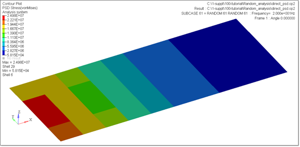
| 5. | Select result type PSD STRESS (t), vonMises, and click Apply. The PSD vonMises stress contour at frequency 20.0 Hz are displayed as below: |

| 6. | Change the Simulation to Simulation 1. |
| 7. | Select the result type RMS stress, vonMises, and click Apply. The RMS stress contour is displayed. |
| 8. | In the HyperView window, click File > Open > Sessions. The Open Session File window opens. |
| 9. | Select the directory where the job was run and select the file direct_psd_rand.mvw. |

See Also:
OptiStruct Tutorials


