|
»Click here to display Table of Contents«
|

Rotating Shell Example |

|

|

|

|
|
Rotating Shell Example |
|
|
|

|
|
»Click here to display Table of Contents«
|
Rotating Shell Example |
|
|
|
|
|
Rotating Shell Example |
|
|
|
|
In some models, the rate of change for the response value with respect to time is very high, and the response is dominant in the design process; this is the case in the following example. The model is a rotating shell structure. A lumped mass is attached to the center of the right hole. The mass of the structure is to be minimized. The driving motion is a rotational velocity at the center of the left hole. Its profile is shown below. The movement of the structure is like the second hand of a watch. Stress of all the elements must be less than an allowable value. Four shape design variables are controllable.
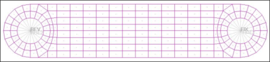
Rotating shell
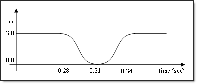
Profile of the driving motion.
After analyzing the initial model, the time history of stress using HyperView can be seen.
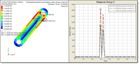
Analysis result of the initial design
According to the analysis result image shown above, the peaks of stress are at around 0.3 seconds. Since the values of these peaks are the largest, you can expect that the responses at around 0.3 seconds will be dominant in the design process. It is a good practice to "zoom in" on the time period around 0.3 seconds so that the optimization process can consider more precise responses. General steps to address the process in this case follow:
| 1. | Run an analysis model with reasonable number of steps in MBSIM card. |
ANALYSIS
$
DESOBJ(MIN)=1
$
SUBCASE 1
MBSIM = 10
MOTION = 11
DESSUB = 11
SPC = 10
:
:
MBSIM 10 TRANS END 0.7 NSTEPS 100
Now you can find out the behavior of the structure as in the analysis result image.
| 2. | According to the results post-processed by HyperView, the maximum stresses are developed at around 0.3 seconds. Increase the number of time steps around 0.3 seconds. That is, divide the time period of 0.28 seconds – 0.34 seconds into 200 steps. Increasing the number of time steps in this period provides the optimizer with more information. |
The element that has the maximum stress and the corresponding time can be changed as the design changes. Thus, Step 2 does not always work. If the time when maximum stress is developed and corresponding element are expected to change dramatically as the design changes, it is best to consider the changed peak time and corresponding element as much as possible.
| 3. | Replace the previous single MBSIM card with multiple MBSIM cards as the following. |
MBSIM 1 TRANS END 0.28 NSTEPS 50
+ VSTIFF
MBSIM 2 TRANS END 0.34 NSTEPS 200
+ VSTIFF
MBSIM 3 TRANS END 0.70 NSTEPS 50
+ VSTIFF
MBSIM 4 TRANS END 1.0 NSTEPS 100
+ VSTIFF
MBSEQ 10 1 2 3
| 4. | Run the optimization problem by removing ANALYSIS command. |
$ANALYSIS
DESOBJ(MIN)=1
$
SUBCASE 1
MBSIM = 10
MOTION = 11
DESSUB = 11
SPC = 10
:
:
MBSIM 1 TRANS END 0.28 NSTEPS 50
+ VSTIFF
MBSIM 2 TRANS END 0.34 NSTEPS 200
+ VSTIFF
MBSIM 3 TRANS END 0.70 NSTEPS 50
+ VSTIFF
MBSEQ 10 1 2 3
Using the above steps, the design process convergence can be enhanced.
The input file can be found in <install_directory>/demos/hwsolvers/optistruct/rotating_shell_design.fem.