The following image shows a cross-section of a typical hydromount:
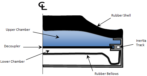
At low displacement amplitudes, fluid in the upper chamber simply deflects the decoupler. The hydromount behaves just like a rubber bushing. As the input displacement increases, the fluid in the upper chamber flows into the lower chamber. With increasing displacement, fluid effects start to dominate and the behavior of the hydromount changes dramatically.
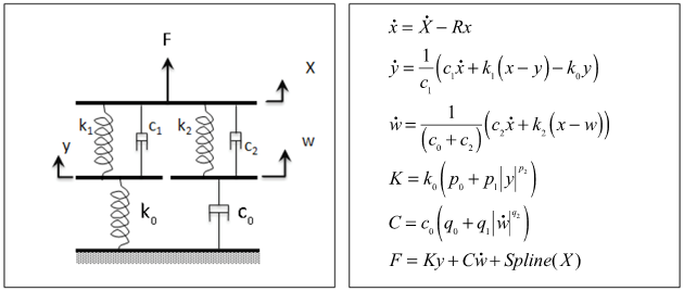
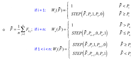
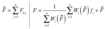
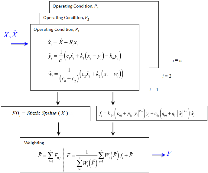
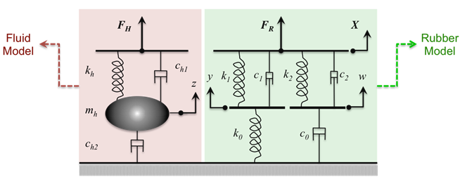
The hydromount model therefore consists of two components: a rubber model and a fluid model. The total response of the hydromount is the sum of the rubber and the fluid effects. A cubic step function gradually turns on the fluid effects, so that transition from rubber behavior to full hydromount behavior is handled correctly. The following figure shows an equivalent mechanical model for the hydromount:
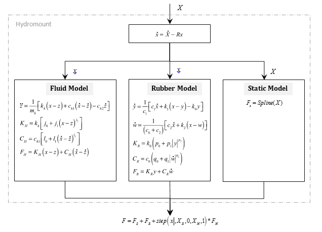
The governing equations for the hydromount model are as follows:
Inputs
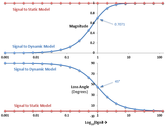
| • | X is the input displacement provided to the bushing. |
| • | R is the cutoff frequency associated with a first order filter. |
| • | The filter removes the steady state deformation of the bushing and passes only the transient portion of the input, x, to the dynamic models. The full input, X, is channeled to the static model. |
Outputs
The total force generated by the bushing is the sum of three forces:
| • | The force due to the fluid behavior, FH, which is turned on gradually. |
| • | The force due to deformation in the rubber component, FR. |
| • | The static force at the operating point, which is computed from the static spline that is provided. |
XR is a design parameter that defines the deformation at which the fluid force transition begins.
XH is a design parameter that defines the deformation at which the fluid force transition ends.
Quite often, the test data for a hydromount does not capture the transition from pure rubber to full hydromount behavior. XR and XH are therefore not fitted, and are available for you to modify in the .gbs. The default values of XR and XH are such that the STEP function always returns 1.0.
For the fluid equations in the center:
| • | z is an internal state representing fluid motion. |
| • | mh represents the equivalent fluid mass. |
| • | kh is the coupling stiffness between rubber and fluid. |
| • | ch1 is the coupling damping between rubber and fluid. |
| • | ch2 is the fluid damping. |
| • | jo, j1, j2 and l0, l1, l2 model the amplitude dependence in the fluid equations. |
| • | KH is the effective fluid stiffness in the bushing. |
| • | CH is the effective fluid damping in the bushing. |
For the rubber equations in the center:
| • | y and w are the internal states of the bushing. |
| • | k0 and k1 represent the bushing stiffness. |
| • | k2 is used to control the stiffness at large velocities. |
| • | c0 produces the roll-off observed in the experimental data at low velocities. |
| • | c1 accounts for the relaxation of the bushing impact force. |
| • | c2 represents the viscous damping observed at large velocities. |
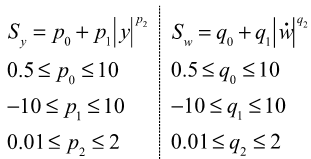
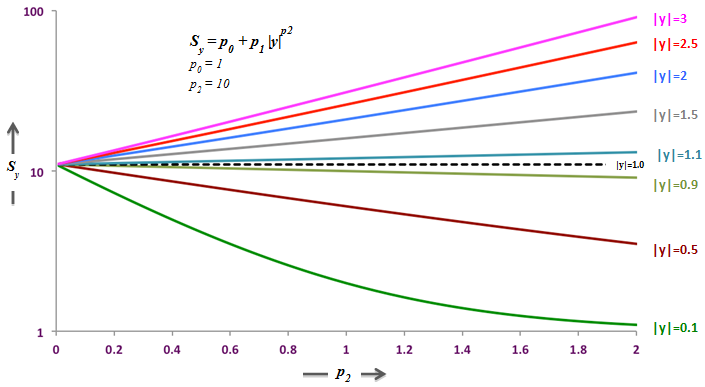
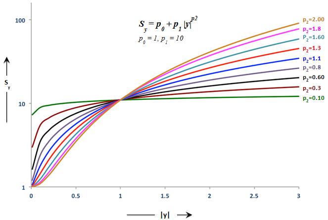
| • | po, p1 , p2 and q0, q1, q2 model the amplitude dependence in the rubber equations. |
| • | K is the effective stiffness of the bushing. |
| • | C is the effective damping of the bushing. |
For the static equations on the right:
| • | Spline (X) is the static force response of the bushing. |
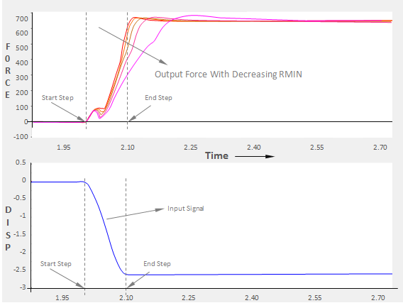
Filter implementation, multiple preload support, and the use of RMIN are exactly the same as for the rubber bushing.
|