Stiffness Force Models

The Altair Bushing Model includes Stiffness Force Models for Spline Stiffness, Constant Stiffness and Cubic Stiffness:

The spline stiffness formulation interpolates a Force vs. Deflection table using Akima’s cubic interpolation method. See reference 4. For values of deflection outside the supplied range, the force is linearly extrapolated using the slope at the corresponding end-point. For each direction employing the spline-stiffness formulation, you must supply a Force vs. Deflection table in the property file. The force is calculated as follows:

Fi=Akispl(qi, table)

Where:

qi	is the displacement of Body-I relative to Body-J in the i th direction after offset, scaling and coupling effects have been considered.
table	is the force-deflection table specified in the [SPLINE_STIFFNESS_xx] block in the .gbs file.

The linear stiffness force is computed according to Hooke’s Law of Elasticity:

Where:

ki	is the constant stiffness value found in corresponding [CONSTANT_STIFFNESS_xx] block for the ith direction in the property file.
qi	is the displacement of Body-I relative to Body-J in the ith direction after offset, scaling and coupling effects have been considered.

The default value for ki is the slope of the experimentally measured static spline at (0,0).

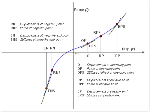
The cubic stiffness force is computed from two cubic-polynomials whose coefficients are determined from the following data:

•	Deflection (O), force (OF), and stiffness (OS) at an operating point.

•	Force and deflection at the point to the left (RN, RNF) and to the right (RP, RPF) of the operating point.

•	Stiffness at the end points to the left (EN, ENS) and right (EP, EPS).

The first cubic polynomial spans the range [O, EP], and the second spans the range [EN, O]. The figure below illustrates the inputs and the resultant curve:

bushing_sim_forc_torque_diagram_mv