HVVH-6000: Solution Tab

In this tutorial, you will learn how to:

•	Check run a solver deck (RADIOSS or OptiStruct).

•	After a check run, compare OUT files of OptiStruct-written result files.

Three options are available for the solver Check Run.

1.	Two OUT files generated from the solver run (RADIOSS or OptiStruct) can be compared.

2.	The current solver run OUT file can be compared with the reference OUT file.

3.	Two OUT files generated from the same solver deck using two different solver versions can be compared.

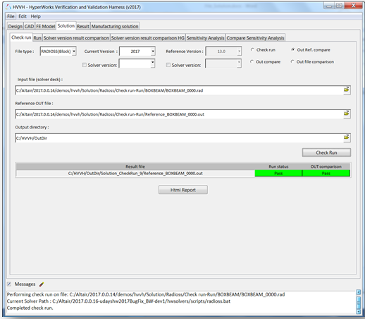
Step 1: Check run solver data for a RADIOSS deck.

1.	From the Solution tab, select the Check run tab.

2.	Activate the Check run option.

hvvh_tut_6000_img1

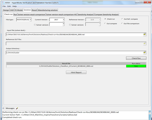
3.	For File type, select RADIOSS(Block).

4.	For Current version, select 2017.

5.	Under Input file, use the file browser icon, , to select and open the following file:

..\tutorials\hvvh\Solution\Radioss\Checkrun\BOXBEAM\BOXBEAM_0000.rad

6.	For the Output directory field, use the open file icon, , to select an output directory.

7.	Click Check Run.

After the check run is complete, the status of the run is displayed in the Messages window.

8.	In the Messages window, the run details are displayed along with the log file location.

9.	Errors are indicated with the label Fail, otherwise, they are labeled Pass.

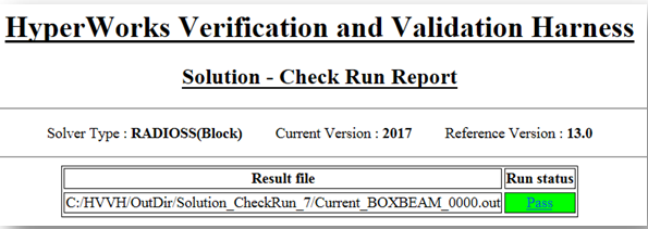
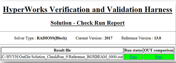
10.	Click HTML Report to view the HTML report.

hvvh_tut_6000_img2

Step 2: Using the Out Compare option.

OUT files generated from the RADIOSS solver check run can be directly compared.

hvvh_tut_6000_img3

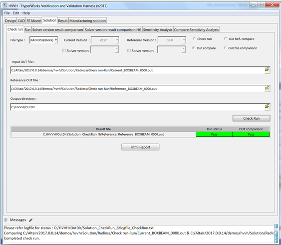
1.	From the Solution tab, select Check Run.

2.	Activate the Out Compare option.

2.	For File type, select RADIOSS(Block).

3.	Under Input OUT file, use the file browser icon, , to select and open the following file:

..\tutorials\hvvh\Solution\Radioss\Checkrun\Current_BOXBEAM_0000.out

5.	Under Reference OUT file, use the file browser icon, , to select and open the following file:

..\tutorials\hvvh\Solution\Radioss\Checkrun\Reference_BOXBEAM_0000.out

6.	For the Output directory field, use the open file icon, , to select an output directory.

7.	Click Check Run.

The OUT files selected are compared, including some of the important blocks in the OUT files. More blocks will be added in later versions of HVVH.

After the Check run (OUT file comparison), the status of the comparison is displayed in the Messages window.

8.	In the Messages window, the run details are displayed along with the log file location.

9.	Differences are indicated with the label Fail, otherwise, they are labeled Pass.

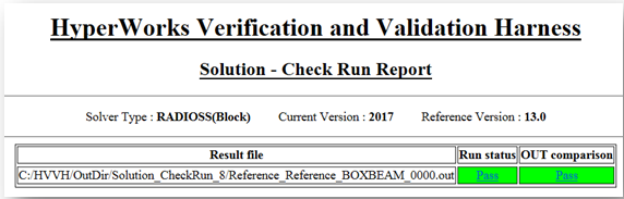
10.	Click HTML Report to view the HTML report. The comparison of different blocks of results are shown line-by-line. Warnings are in light orange and errors are in dark orange.

hvvh_tut_6000_img4

Step 3: Use the Out Ref. Compare option.

Out files generated from the solver check run can be compared with the reference OUT file.

hvvh_tut_6000_img5

1.	From the Solution > Check run tab, activate the Out Ref. compare option.

2.	For File type, select RADIOSS(Block).

3.	For Current version, select 2017.

4.	Under Input file, use the file browser icon, , to select and open the following file:

..\tutorials\hvvh\Solution\Radioss\Checkrun\BOXBEAM\BOXBEAM_0000.rad

This file is used for the solver run in the background.

5.	Under Reference OUT file, use the file browser icon, , to select and open the following file:

..\tutorials\hvvh\Solution\Radioss\Checkrun\Reference_BOXBEAM_0000.out

This file is used to compare the first generated OUT file.

6.	For the Output directory field, use the open file icon, , to select an output directory.

7.	Click Check Run.

The generated OUT file and reference OUT files are compared, including some of the important blocks in the OUT files are compared. More blocks will be added in later versions.

8.	After the Check run (OUT file comparison) is complete, the status of the comparison is displayed in the Messages window.

9.	In the Messages window, the run details are displayed along with the log file location.

10.	Differences are indicated with the label Fail; otherwise, they are labeled Pass.

11.	Click HTML Report to view the HTML report. The comparison of different blocks of results are shown line-by-line. Warnings are in light orange and errors are in dark orange.

hvvh_tut_6000_img6

Step 4: Using the Out file comparison option.

Out files generated from different solver versions can be directly compared.

hvvh_tut_6000_img7

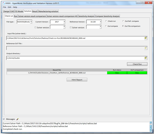
1.	From the Solution > Check run tab, activate the Out file comparison option.

2.	For File type, select RADIOSS(Block).

3.	For Current version, select 2017.

4.	For Reference version, select 14.130.

5.	Under Input file, use the file browser icon, , to select and open the following file:

..\tutorials\hvvh\Solution\Radioss\Checkrun\BOXBEAM\BOXBEAM_0000.rad

This is the solver file that will be used to run the solver for the check run. The OUT file is created in the output directory.

6.	For the Output directory field, use the open file icon, , to select an output directory.

7.	Click Check Run.

The generated OUT files are compared, including some of the important blocks in the OUT files. More blocks will be added in later versions.

8.	After the check run (OUT file comparison) is complete, the status of the comparison is displayed in the Messages window.

9.	In the Messages window, the run details are displayed along with the log file location.

10.	Differences are indicated with the label Fail; otherwise, they are labeled Pass.

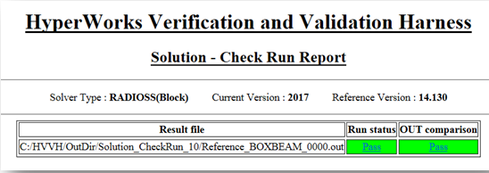
11.	Click HTML Report to view the HTML report. The comparison of different blocks of results are shown line-by-line. Warnings are in light orange and errors are in dark orange.

hvvh_tut_6000_img8

Step 5: Solver run.

After a complete solver run, you can compare OUT files for solver-written result files.

Three options are available for the OUT file comparison under the Run option of the solver.

1.	Two OUT files generated from the solver run can be compared.

2.	The current solver run OUT file can be compared with the reference OUT file.

3.	Two OUT files generated from the same solver deck using two different solver versions can be compared.

hvvh_tut_6000_img9

Begin the tutorial:

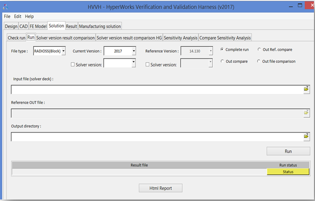
1.	From the Solution > Run tab, activate the Complete run option.

2.	For File type, select RADIOSS(Block).

3.	For Current version, select 2017.

4.	Under Input file, use the file browser icon, , to select and open the following file:

..\tutorials\hvvh\Solution\Radioss\Run\BOXBEAM\BOXBEAM_0000.rad

This file is used for the solver run in the background.

5.	For the Output directory field, use the open file icon, , to select an output directory.

6.	Click Run.

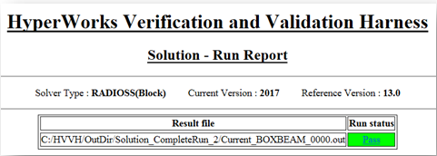
After the run is complete, the status of the comparison is displayed in the Messages window.

7.	In the Messages window, the run details are displayed along with the log file location.

8.	Errors are indicated with the label Fail; otherwise, they are labeled Pass.

9.	Click HTML Report to view the HTML report.

hvvh_tut_6000_img10

10.	The following three options on the Run tab work as they do on the Check run tab (see Steps 2-4 above).

•	Out compare (out files comparison)

•	Out Ref. compare (out files comparison)

•	Out file comparison from solver check runs

For RADIOSS, both the Starter OUT file and Engine OUT files are compared.

For OptiStruct, the OUT files are compared.

Step 6: Solver version result comparison (RADIOSS or OptiStruct)

In this section, you will use the Solver version result comparison option for a given model. If the result files are not available, the Solver Run can be done in the background and the result generated are used in the result comparison.

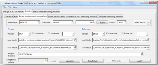
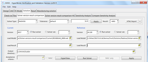
1.	From the Solution tab, select the Solver version result comparison tab.

hvvh_tut_6000_img11

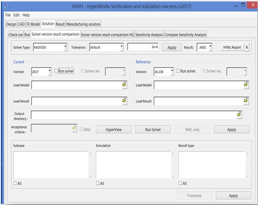
2.	For Solver type, select RADIOSS.

3.	For Tolerance, select the default (1e-06). You can set any tolerance for Scalar, Vector, or Tensor data types.

4.	For Result, select A001.

5.	Click HTML Report.

6.	Under Current, for Load Model, use the file browser icon, , to select and open the following file:

..\tutorials\hvvh\Solution\Radioss\Solver-versions-result-comparison\Current\BOXBEAM_0000.rad file.

7.	Under Reference, for Load Model, use the file browser icon, , to select and open the following file:

..\tutorials\hvvh\Solution\Radioss\Solver-versions-result-comparison\Reference\BOXBEAM_0000.rad file.

8.	For the Output directory field, use the open file icon, , to select an output directory.

hvvh_tut_6000_img12

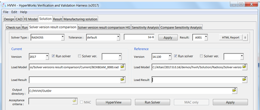
9.	Activate the Run solver options.

10.	Click Run Solver.

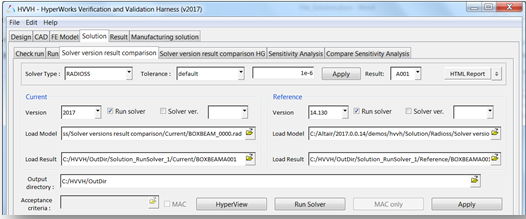
After the solver run, the A001 results are loaded in the Load Result option.

hvvh_tut_6000_img13

11.	Click Apply.

The results available (Subcase, Simulation, and Result type) in the current result file are loaded in the three windows.

hvvh_tut_6000_img14

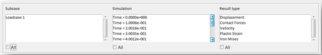
12.	Select each All under each of the windows and click the second Apply button.

Any combination of Subcase, Simulation, and Datatype can be selected for comparison.

Results comparison of the current and reference results are generated.

13.	In the Messages window, the run details are displayed along with the log file location.

14.	If any difference is greater than the tolerance, it is indicated with the label Fail, otherwise, they are labeled Pass.

hvvh_tut_6000_img15

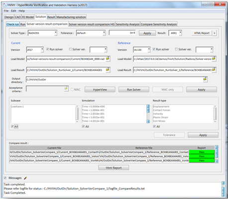
15.	Click HTML Report to view the HTML report. Comparisons between different data types are available.

For example, for a vector (Displacement), the components Magnitude, X-displacement, Y-displacement, and Z-displacement are compared for the entire model and results are displayed.

hvvh_tut_6000_img16

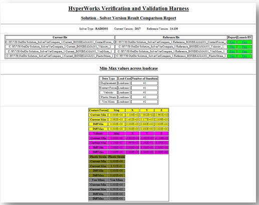
16.	Click Pass/Fail in the HTML report to open a detailed comparison report.

The second column in the table, Launch HV, opens HyperView. Depending on the data type, different windows are opened with the respective diff results.

For example, for vector results (Displacement), four windows open with the Magnitude, Displacement –X, Displacement –Y, and Displacement –Z loaded in the different windows. In each window, further details can be viewed.

17.	Click the first column of the table to open a new graphics window.

hvvh_tut_6000_img17

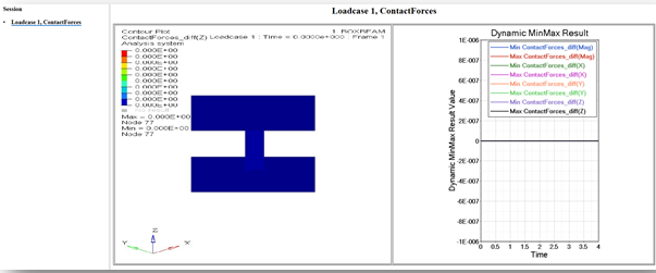
In the image above, the left window shows a diff contour (Current-Reference) and the right window shows a diff plot in HyperGraph.

18.	In case any difference is greater than the tolerance, it is indicated with the label Fail, otherwise, it is labeled Pass.

19.	Click the left window to open the diff-values H3D in HyperView Player. You can view the difference in the contour and view the area where there is a difference in case of a failure.

20.	Click the right window to maximize/minimize the plot. The difference values for each step are calculated and the min and max values of the difference are plotted.

If all the values match and no difference is seen, the curve is a flat line and the diff contours have values less than the tolerance.

Step 7: Solver version result comparison (HyperView option - HyperView interactive)

1.	From the Solution tab, select the Solver version result comparison tab.

hvvh_tut_6000_img18

2.	For the Solver Type, select RADIOSS.

3.	For Tolerance, select the default (1e-06). You can set any tolerance for the Scalar, Vector or Tensor data types

4.	For Result, select A001.

5.	Click HTML Report.

6.	For Current Version, select 2017.

7.	For Reference Version, select 14.130.

8.	Under Current, for Load Model, use the file browser icon, , to select and open the following file:

..\tutorials\hvvh\Solution\Radioss\Solver-versions-result-comparison\Current\BOXBEAM_0000.rad

9.	Under Reference, for Load Model, use the file browser icon, , to select and open the following file:

..\tutorials\hvvh\Solution\Radioss\Solver-versions-result-comparison\Reference\BOXBEAM_0000.rad

10.	For the Output directory field, use the open file icon, , to select an output directory.

11.	Activate the Run solver options.

12.	Click Run Solver.]

After the solver run, the A001 results are loaded in the Load Result option.

hvvh_tut_6000_img19

13.	Click HyperView.

Hyperview opens the current results and reference results and loads them into two windows.

14.	Model and results are pre-loaded for both the current and reference models in HyperView. From the Contour panel, select data type and data component.

15.	Control is active for first window.

•	Select a region of interest (element, node, component level) and create a contour.

•	Run the command ::Displaycontour (reference result contour is also loaded for the selected region).

•	Run a command to apply a user-defined tolerance for the data type selected ::Applytolerance (otherwise, use the default tolerance).

•	Run the command ::Diffcontour. Difference contour result are displayed in another window for the selected data types only and are also plotted.

hvvh_tut_6000_img20

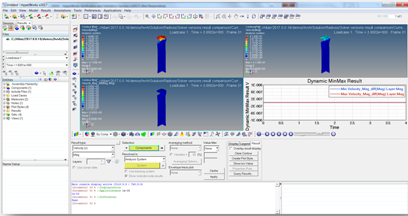
16.	The first window displays the current model and result, and the second window displays reference model and result.

17.	The third window displays the difference in the contour values. If the difference is greater than the tolerance, it is indicated as Fail, otherwise its displayed as Pass.

18.	The fourth window displays the actual diff plots in HyperGraph.

The data type can be changed and any individual component result can be compared. Tolerance values can be reset to any value and result comparison.

Comparison for region of interest:

•	Part of the model (by window, by component, set of elements, and so on) can be selected in the first window. Using APIs as mentioned above, results can be compared ONLY for the selected region.

Step 8: Solver version result comparison HG

In this step, you will compare results from different solver versions (RADIOSS or OptiStruct) using HyperGraph.

1.	From the Solution tab, select Solver version result comparison HG.

hvvh_tut_6000_img21

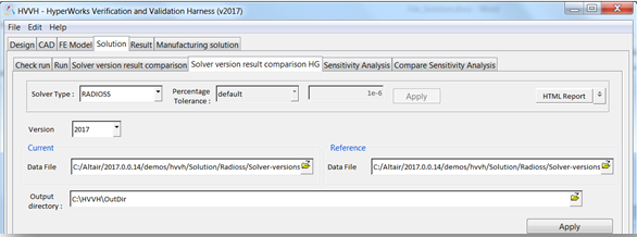
2.	For Solver Type, select RADIOSS.

3.	Click HTML Report.

4.	For Version, select 2017.

5.	Under Current, for Data File, use the file browser icon, , to select and open the following file:

..\tutorials\hvvh\Solution\Radioss\Solver-versions-result-comparison-HG\Current_BOXBEAMT01

6.	Under Reference, for Data File, use the file browser icon, , to select and open the following file:

..\tutorials\hvvh\Solution\Radioss\Solver-versions-result-comparison-HG\Reference_BOXBEAMT01

7.	For the Output directory field, use the open file icon, , to select an output directory.

8.	Click Apply.

hvvh_tut_6000_img22

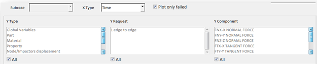
9.	Select each All and click the second Apply.

Any combination of the Y-Type, Y Request, and Y Component can be selected for comparison.

10.	In this example, the solver result for the same model with slightly different Boundary conditions are picked to show the difference in the results so that they are visible in the graphs of the report.

Results comparison of the current results and reference plot results are generated.

11.	In the Messages window, the run details are displayed along with the log file location.

hvvh_tut_6000_img23

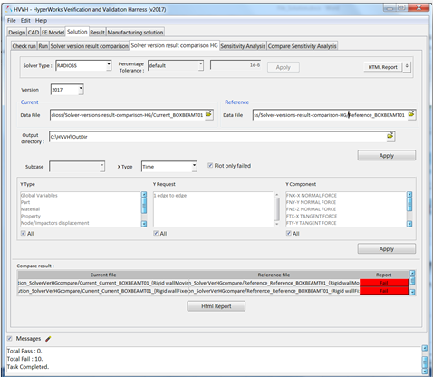
12.	Click HTML Report to open the report. Comparison of different Types, Requests, and Components (TRC) are available.

hvvh_tut_6000_img24

hvvh_tut_6000_img25

hvvh_tut_6000_img26

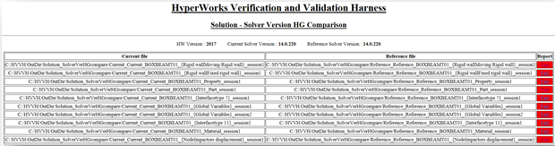
13.	Click the Fail in HTML report to open a detailed comparison report.

Here, the boundary conditions are different and there is a difference in results.

14.	Click on the plots to maximize/minimize the images.

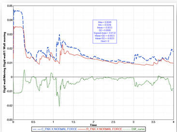
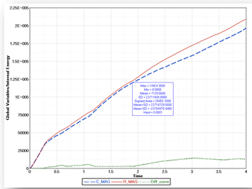
15.	Graphs display the current and reference curves along with the difference curve.

16.	The diff curve shows differences in current/reference curves. Any non-zero diff value is a failure.

17.	All statistical details of the difference curve is also shown in the graph table.

Step 9: Sensitivity Analysis.

Compare results from different solver versions (RADIOSS or Optistruct) using Sensitivity Analysis. Sensitivity analysis of the model is carried out for different seed values.

1.	From the Solution tab, select the Sensitivity Analysis tab.

hvvh_tut_6000_img27

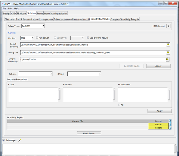
2.	For Solver Type, select RADIOSS.

3.	Click HTML Report.

4.	For Version, select 2017.

5.	Activate the Use existing results option.

The results of from a previously run solver analysis is used.

6.	For Result directory, use the file browser icon, , to browse here:

..\tutorials\hvvh\Solution\Radioss\Sensitivity-Analysis

7.	For Config File, use the file browser icon, , to select and open the following file:

..\tutorials\hvvh\Solution\Radioss\Sensitivity-Analysis\config_thickness_0.txt

This file is used to set different seed values for the sensitivity analysis.

8.	For the Output directory field, use the open file icon, , to select an output directory.

9.	Click Apply.

hvvh_tut_6000_img28

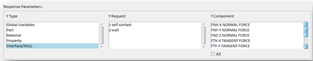
10.	Under Response Parameters, select TRCs for the sensitivity study and click Apply.

The sensitivity report is generated.

11.	In the Messages window, the run details are displayed along with the log file location.

hvvh_tut_6000_img29

12.	Click HTML Report to open the sensitivity report.

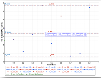
13.	In the HTML report for one TRC, there will be two reports.

1.	Seed Vs TRC.

This is a scattered plot, showing sensitivity for each seed value. This creates a sensitivity corridor that can be used to study the variation or sensitivity of the result for the given model.

2.	Time Vs TRC.

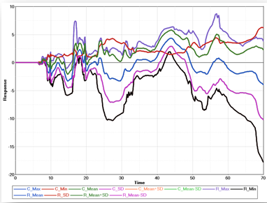
This shows:

- All Time History (TH) plots across the seed values.

- Envelope cures (Max, Min, Mean, SD, Mean+SD, and Mean-SD).

- Statistical curves (Max, Min, Mean, SD, Mean+SD, and Mean-SD).

The detailed report points to different sets of information to help you further assess the results and perform the sensitivity study, and if this model can be used further for solver version result comparisons.

Step 10: Compare results from different Solver versions (RADIOSS or OptiStruct) using Sensitivity analysis.

Actual solver version result comparison for solver plot results using this sensitivity analysis, carried out using different solver versions for the same model.

1.	From the Solution tab, select the Compare Sensitivity Analysis tab.

hvvh_tut_6000_img30

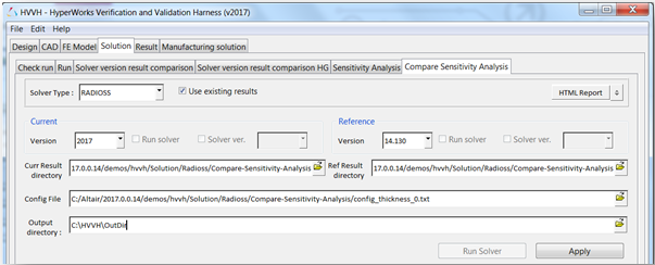
2.	For Solver Type, select RADIOSS.

3.	Activate the Use existing results option.

4.	Click HTML Report.

5.	For Current Version, select 2017.

6.	For Reference Version, select 14.130.

7.	For Current Result directory, use the file browser icon, , to browse to the following location:

..\tutorials\hvvh\Solution\Radioss\Compare-Sensitivity-Analysis

8.	For Reference Result directory, use the file browser icon, , to browse to the following location:

..\tutorials\hvvh\Solution\Radioss\Compare-Sensitivity-Analysis

9.	For Config File, use the file browser icon, , to select and open the following file:

..tutorials\hvvh\Solution\Radioss\Compare-Sensitivity-Analysis\config_thickness_0.txt

10.	For the Output directory field, use the open file icon, , to select an output directory.

11.	Click Apply.

hvvh_tut_6000_img31

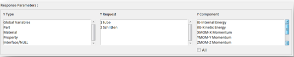
12.	Select each All under the Type, Request, and Component (TRC) windows and click the second Apply button.

The sensitivity report is generated for comparison across two versions.

13.	In the Messages window, the run details are displayed along with the log file location.

hvvh_tut_6000_img32

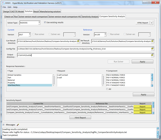
14.	Click HTML Report to open the sensitivity report.

hvvh_tut_6000_img33

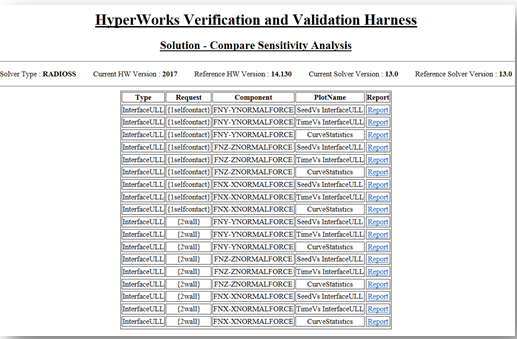
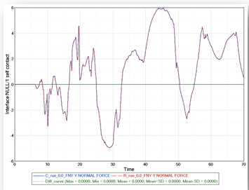
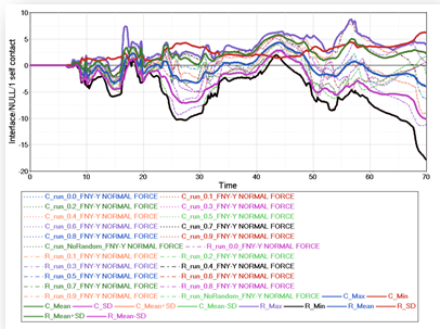
15.	In the HTML report for one TRC, there will be two reports. For each of the solver results from different solver versions, the results are extracted and plotted for comparison.

1.	Seed Vs TRC.

This is a scatter plot, showing sensitivity for each seed value. Using this sensitivity corridor, the variations across different seed vales for results from two solver versions can be determined.

2.	Time Vs TRC.

This shows Time History (TH) plots for the current and reference files and their diff curve.

3.	Curve Statistic

- Envelop of all cures (Max, Min, Mean, SD, Mean+SD, and Mean-SD).

- Statistical curves (Max, Min, Mean, SD, Mean+SD, and Mean-SD).

hvvh_tut_6000_img34

hvvh_tut_6000_img35

hvvh_tut_6000_img36

hvvh_tut_6000_img37