Altair Driver is a simple driver model. This is used in all MotionView and MotionSolve vehicle events. The controller can predict the future road path based on the current vehicle state, has knowledge of the vehicle dynamics, and has access to user-defined driver parameters.
Input driver parameters specify the control priorities of the driver. Vehicle parameters are used to estimate the vehicle’s future states, based on a simple linear bicycle model. The following paragraphs describe vehicle and driver parameters and their effects on the trajectory planning.
Usage
Altair Driver is implemented as a user-defined solver variable. Its value is then used in the steering system motion statement. When a vehicle event is selected from the Analysis Wizard in MotionView, the driver is automatically added to the multi-body model as are the required entities (arrays, solver variables, and so on).
Theory
The well-known bicycle model is used as a first approximation to represent a four-wheeled road vehicle.
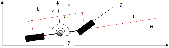
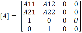
With some approximations, the equations on motion can be easily written in the form:
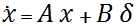
Where the state vector is:
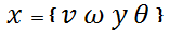
The quantities are:
| • |  Vehicle Yaw angle Vehicle Yaw angle |
| • |  Lateral speed of the vehicle (side slip) Lateral speed of the vehicle (side slip) |
| • |  Yaw rate of the vehicle Yaw rate of the vehicle |
| • | y Lateral position of the vehicle CG on the global axes |
and
| • |  Road wheel steer angle (directly proportional to the steering wheel angle by a rack/pinion reduction ration factor). Road wheel steer angle (directly proportional to the steering wheel angle by a rack/pinion reduction ration factor). |
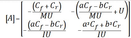
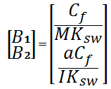
The A and B matrices can be calculated using Newton’s second law of motion and, with the assumption of small angles (sin 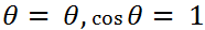 ) they become:
Once the equations of motion have been written, the problem becomes that of classical control theory. The goal is to calculate the steering wheel angle that would cause the vehicle to follow a prescribed path as closely as possible.
This can be achieved in many different ways. One strategy could be to use optimal control theory and minimize a cost function measuring a series of weighted factors (including lateral position error, hand-wheel steering angle, and heading error) evaluated at different time steps.
With Altair Driver, MotionSolve computes the error between the predicted path and the desired path at some point in the future. The controller has full knowledge of the vehicle dynamics equations as described above and is able to compute the predicted position based on those equations at some future time.
To compute the predicted path, the equations of motion are integrated at look-ahead times by using the Runge-Kutta integration scheme. The path is obtained by spline interpolation using the GTCURV utility function in MotionSolve.
The difference between the predicted path and desired path at look-ahead is the error.
Thus:

The algorithm attempts to estimate the error by evaluating its sensitivity to the steering wheel angle. Convergence is achieved when the error is less than a certain tolerance.
The final steering wheel angle is calculated by the iterative method described below:
| 1. | Two appropriate steering wheel angle values are chosen and called  and and  . . |
| 2. | The corresponding errors  and and  are calculated and a steering wheel angle, are calculated and a steering wheel angle,  , is chosen by linear interpolation using the following formula: , is chosen by linear interpolation using the following formula:
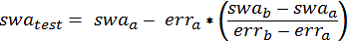 |
| 3. | If the error corresponding to the steering wheel angle is less than a certain tolerance, then it is used as the steering wheel angle at the next time step. |
| 4. | If the error corresponding to the steering wheel angle is more than the tolerance, then the or which resulted in more error is replaced by and Step 2 is performed again. |
Note that for the first integration step, is chosen as the current steering angle and is the current steering angle plus 1 degree. Finally, if the steering wheel angle does not converge after 20 iterations, an error is thrown and the simulation is stopped, signaling the fact that the vehicle cannot perform the path following maneuver.
The final steering wheel angle is essentially used as an increment to the current steering wheel angle as shown below. When computing the new steering wheel angle value (at time t+1), the previous value of the steering wheel angle (at time t) is updated by the quantity:

Where:
| • |  is the step size (the difference between the last successful integration time and the current time). is the step size (the difference between the last successful integration time and the current time). |
| • |  is the feedback frequency which captures the driver reaction times (should be less than the step frequency). is the feedback frequency which captures the driver reaction times (should be less than the step frequency). |
Limitations
Since the controller uses a simplified linear representation of the vehicle, its applicability is limited to the linear range. Another simplification done to the equations is that of small angles (yaw angle). This means that the stability and the accuracy of the controller decrease greatly for vehicles performing maneuvers outside of the linear range.
User Inputs
You can enter vehicle parameters and driver parameters by defining two arrays. The vehicle parameter array contains quantities that are used in the definition of the bicycle model.
These include:
| • | Rear WC to CG long distance (b) |
| • | Front WC to CG long distance (a) |
| • | Front tire cornering stiffness ( ) ) |
| • | Rear tire cornering stiffness ( ) ) |
| • | Steering ratio (hand-wheel to front-wheel angle gain,  ) ) |
The driver parameter array defines quantities that influence the driver behavior, as well as all the markers used to compute all the vehicle kinematic states.
These include:
| • | Feed frequency value () [-] |
| • | Maximum steering wheel angle [deg] |
| • | Path origin ID (usually a marker on the road coincident with the vehicle body CM) |
The maximum steering wheel angle is ultimately used as cut-off value for the computed steering wheel angle.


