MV-1012: Analytical Contact Simulation Using MotionView and MotionSolve

In this tutorial, you will learn how to:

•	Setup semi-analytical contact between a primitive spherical geometry and a meshed geometry.

•	Perform a transient analysis to calculate the contact forces between these geometries.

•	Process the results.

•	Compare the analysis time when using meshed representation for the spheres.

For these purposes, you will make use of a ball bearing model.

Introduction

This tutorial will guide you through the new analytical 3-D rigid body contact capabilities in MotionSolve. When one or both of the rigid bodies in contact are primitive spheres, MotionSolve uses a semi-analytical or fully analytical contact method respectively to calculate the penetration depth(s) and subsequently the contact force(s). This is explained in the table below:

Body I graphic	Body J graphic	Contact method	Description
Primitive Sphere	Mesh	Sphere – Mesh	A semi-analytical contact method that computes contact between the primitive sphere (Body I) and the tessellated geometry (Body J).
Primitive Sphere	Primitive Sphere	Sphere – Sphere	A fully analytical contact method that is independent of the tessellation of either graphics.

There are several 3D contact applications that involve spherical geometries (ball bearings, re-circulating ball systems etc.) – using the analytical approach for computing the contact forces in such scenarios offers several benefits:

1.	The simulation time is reduced when using the semi-analytical or fully analytical approach.

2.	The simulation is more robust since the dependence on the mesh quality is removed.

3.	The simulation results are often more accurate since there are no or lesser effects of mesh discretization.

Ball Bearing Model

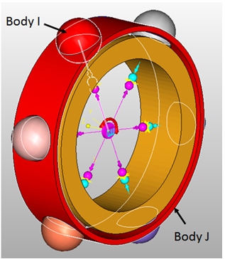
A ball bearing is a type of bearing that consists of balls located between the outer and inner bearing races. The balls are in contact with both the outer and inner races. The purpose of the balls is mainly to support radial loads between the two races while minimizing losses due to friction. Since the balls roll in between the two races, the friction is drastically reduced as compared to two surfaces sliding against each other. A typical ball bearing geometry is illustrated in the figure below:

mv-1012_ball_bearing_model

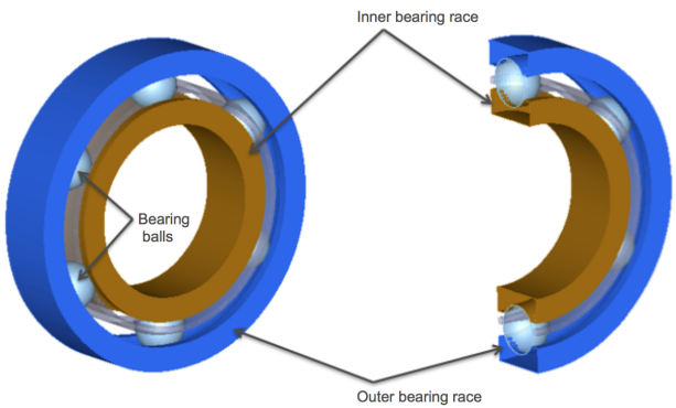
A typical ball bearing geometry with six balls. A cutaway section shows how the balls are in contact with the outer and inner races.

The geometries for all surfaces except the balls are meshed in this geometry. Only the six balls are defined as primitive spheres.

Step 1: Loading the model in MotionView.

1.	Copy the Ball_Bearing.mdl file, located in the mbd_modeling\contacts folder, to your <working directory>.

2.	Start a new MotionView session.

3.	Open the Ball_Bearing.mdl model file from the <working directory>.

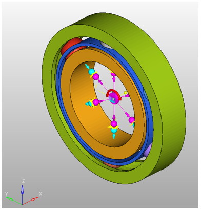
mv-1012_ball_bearing_motionview_model

MotionView model for the ball bearing mechanism

The figure above shows the model as it is setup in MotionView. This model has all the necessary contacts defined except for a few which you will setup next. The following table describes the components present in this model.

Component name	Component type	Description
Ground Body	Rigid body	Ground Body
Outer Race	Rigid body	The outer bearing race body
Inner Race	Rigid Body	The inner bearing race body
Ball 1, , Ball 6	Rigid Body	Ball bodies
Rim	Rigid Body	The rim body that keeps the balls in place
Ball1_inter, …, Ball5_inter	3D rigid body contact	Contact force element between the balls and the Rim
Ball1_upper, …, Ball5_upper	3D rigid body contact	Contact force elements between the balls and the Outer Race
Ball1_inter, …, Ball5_inter	3D rigid body contact	Contact force elements between the balls and the Inner Race
Solver Units	Data Set	The solver units for this model. These are set to Newton, Millimeter, Kilogram, Second
Gravity	Data Set	Gravity specified for this model. The gravity is turned on and acts in the negative Z direction
Outer Race Graphic	Graphic	The graphic that represents the outer race body. This is a tessellated graphic
Inner Race Graphic	Graphic	The graphic that represents the inner race body. This is a tessellated graphic
Rim Graphic	Graphic	The graphic that represents the rim body. This is a tessellated graphic
Ball 1 – Primitive, …, Ball 6 - Primitive	Graphic	The graphics that represent the ball bodies. These are primitive geometries
Inner Race Rev	Revolute Joint	Revolute joint defined between the Inner Race and Ground Body
Outer Race Fixed	Fixed Joint	Fixed joint defined between the Outer Race and Ground Body
Input Motion to Inner Race	Motion	A motion defined on the Inner Race Rev joint that actuates the mechanism

Step 2: Defining contact between the primitive and meshed geometries.

In this step, you will define contact between:

•	Ball 6 and the Outer Race

•	Ball 6 and the Rim

•	Ball 6 and the Inner Race

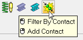
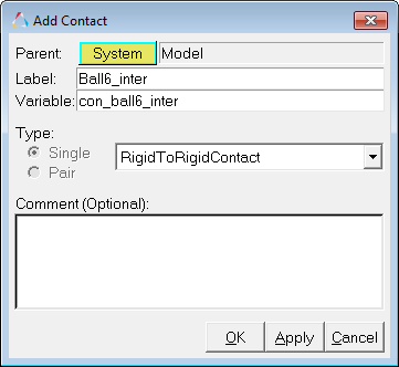
1.	Add a new contact force entity by right-clicking on the Contact button in the Force Entity toolbar:

mv-1012_contact_button

The Add Contact dialog is displayed.

2.	For Label, enter Ball6_inter.

3.	For Variable, enter con_ball6_inter.

4.	Verify that RigidToRigidContact is selected in the drop-down menu and click OK.

mv-1012_add_contact_dialog

The Contact panel is displayed.

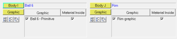
5.	From the Connectivity tab, resolve Body I to Ball 6 and Body J to Rim. This will automatically select the graphics that are attached to these bodies.

mv-1012_contact_panel

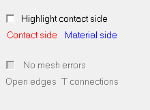
To make sure that the geometries are well defined for contacts, the normals of the surface mesh should be along the direction of contact and there should be no open edges or T-connections in the geometries. To make sure the normals are oriented correctly, activate the Highlight contact side box. This will color the geometries specified for this contact force according to the direction of the surface normals. You should make sure both geometries are completely red i.e. there are no blue patches for either geometry. To see this clearly, you may have to deactivate the Outer Race graphic. This is illustrated in the figures below.

mv-1012_hghlt_cntct_side_option mv-1012_chckng_fr_incrrct_surface_nrmls_example

Checking for incorrect surface normals

Next, you can check for open edges or T-connections. If the associated graphics mesh has any open edges or T-connections, the Highlight mesh errors option would be active. Activate the box for Highlight mesh errors if there are any mesh errors. Doing this will highlight any open edges or T Connections in the geometry.

The graphics associated in this contact entity don’t have mesh errors. Hence you should see Highlight mesh errors grayed out.

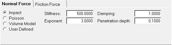
8.	Next, you need to specify the contact properties. To do this, click on the Properties tab to bring up the Normal Force and the Friction Force property tabs within the Contact panel. In this model you will use an Impact model with the following properties:

Normal Force Model	Impact
Stiffness	500.0
Exponent	3.0
Damping	1.0
Penetration Depth	0.1
Friction Force Model	Disabled

Specify the properties as defined above in the contact panel.

mv-1012_normal_force_tab

9.	Repeat steps 1 – 3 for creating contact between the Ball 6 body and the Outer Race body and also between the Ball 6 body and the Inner Race body. The details for these are listed in the table below:

Label	Ball6_outer	Ball6_inner
Variable	con_ball6_outer	con_ball6_inner
Body I graphic	Ball 6 – Primitive	Ball 6 – Primitive
Body J graphic	Outer Race Graphic	Inner Race Graphic
Normal Force Model	Impact	Impact
Stiffness	1000.0	1000.0
Exponent	2.1	2.1
Damping	0.1	0.1
Penetration Depth	0.1	0.1
Friction Force Model	Static and Dynamic	Static and Dynamic
Mu Static	0.4	0.5
Mu Dynamic	0.2	0.3
Stiction transition velocity	1.0	1.0
Friction transition velocity	1.5	1.5

10.	Save your model.

Step 3: Setting up a transient simulation and running the model.

At this point, you are ready to setup a transient analysis for this model.

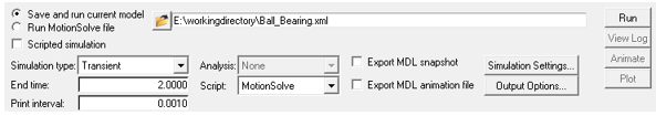
1.	To setup a transient analysis, navigate to the Run panel by clicking on the Run button in the toolbar .

2.	From the Run panel, change the Simulation type to Transient and specify an end time of 2.0 seconds.

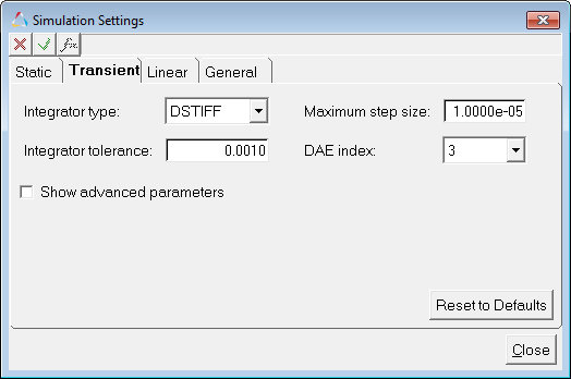
3.	Further, to obtain accurate results, you will need to specify a smaller step size than the default. Click on the Simulation Settings button and navigate to the Transient tab.

4.	Set the Maximum step size to 1e-5 and click Close.

mv-1012_simulation_settings_dialog_transient_tab

5.	Specify a name for your XML model and click the Run button. This will start the transient simulation.

mv-1012_run_panel

6.	In the HyperWorks Solver View window that pops up, a message is displayed from the solver that confirms that the semi-analytical contact method is being used for the contact calculations.

mv-1012_hw_solver_view_dialog

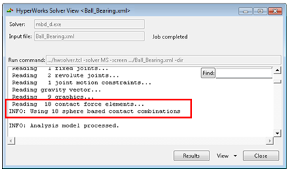
As you may have noticed, you did not have to explicitly specify the contact force method to be used. MotionSolve automatically detects if one or both the bodies in contact are primitive spheres and accordingly changes the contact force method being used.

Step 4: Post-processing the results.

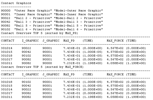
After the simulation is complete, MotionSolve prints out a summary table (both on screen and in the log file generated) that lists the top five contact pairs ordered by maximum penetration depth and by maximum contact force for this simulation. This is very useful since it can be used to verify that the model is behaving as intended even before loading the results (ABF, MRF, PLT or H3D) files. You can also use this table to verify that the penetration depths and contact forces are within the intended limits for your model. The summary table for this simulation is illustrated below:

mv-1012_summary_table_example

1.	Motionview makes available an automated report for model containing contacts. The report automatically adds animation and plots to the session. The report can be accessed through Analysis > View Reports menu option.

mv-1012_analysis_menu_view_reports

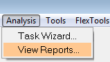
The View Reports dialog is displayed.

2.	The report item, Contact Report, for the last submitted run will be listed at the top. Select that item and click OK.

mv-1012_view_reports_dialog

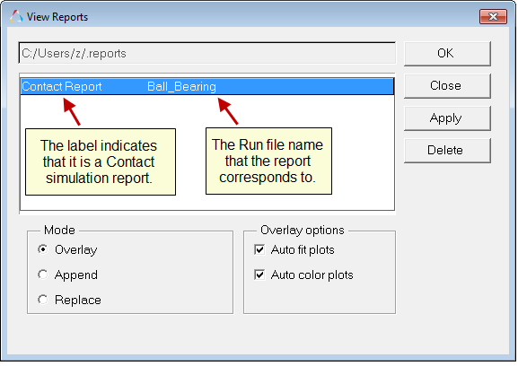
3.	Additional pages are added to the report. Use the Page Navigation buttons (located at the upper right corner of the window, below the menu bar area and above the graphics area) to view these pages.

Contact Overview

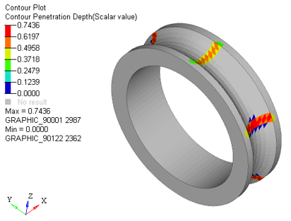
MotionSolve writes out a static load case to the H3D file that can be used to view the maximum penetration on all the geometry in contact throughout the length of the simulation. This enables you to inspect your results to see where the maximum penetration depth occurred in your geometry/geometries. You may hide one or more parts to view this clearly in the graphic area.

Note You may Fit the graphic area in case the graphics are not visible in the Graphics area.

1.	From the Results browser select the components Ball 1 – Primitive to Ball 6 – Primitive.

2.	Right-click and click Hide from the context menu.

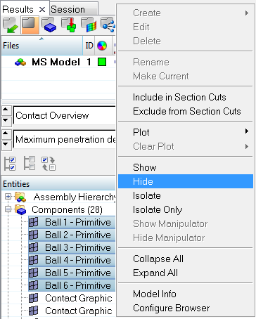
mv-1012_hv_results_browser_hide_option

3.	Similarly, Hide the Rim graphic and Inner Race graphic in order to visualize the contours on the Outer Race graphic.

mv-1012_contour_plot_example

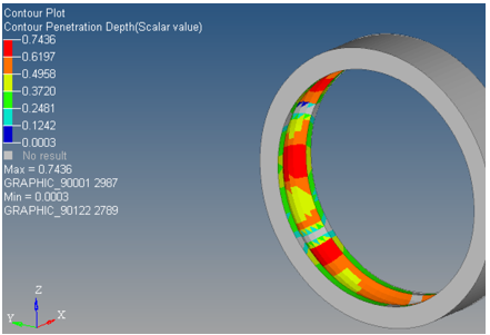
Contact overview for penetration depth

Animation – Penetration Depth

1.	Navigate to the next page , which shows a transient animation of the penetration depth.

2.	You can visualize the contours individually on the components by isolating the components. For example, to visualize the contours on the Inner Race graphic, select the component in the Results browser, right-click and select Isolate from the context menu.

3.	Click on Start/Pause Animation to view the animation.

mv-1012_contour_plot_example2

Visualizing the Contact forces via force vectors

1.	Navigate to the next page , which shows a transient animation of the contact forces.

2.	Fit the model in the graphics area.

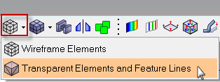
3.	Select Transparent Element and Feature Lines from the toolbar options.

mv-1012_hv_transp_elements_feature_lines

4.	Go to the Vector panel.

5.	Activate the Display tab and change the Size Scaling option to By Magnitude and use a value of 5.

6.	Click on Start/Pause Animation button to view the animation.

mv-1012_vector_plot_example

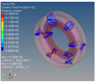
Animating the total contact force (the outer race graphic is turned off for better visualization)

Plotting Contact Forces

mv-1012_hg_plot_example

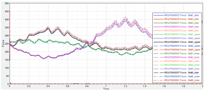
Note	You may turn off curves from the Plot browser to look at individual force plots.

1.	Each time a new contact entity is created in MotionView, a corresponding output force request is created that can be used to plot the contact forces between the geometries specified in the contact entity.

2.	Go to the next page , which has a HyperGraph plot of all the contact force magnitudes.

Step 5: Comparing the run time with a model containing meshed spheres.

The semi-analytical (and fully analytical) contact method is more efficient than the 3D mesh-mesh based contact. To illustrate this, you can run the same model you just created however instead of using primitive spheres for the bearings, use a meshed representation. Such a model is already available in your HyperWorks installation. Copy the model Ball_Bearing_meshed.mdl, located in the mbd_modeling\contacts folder, to your <working directory>. Run this model from MotionView and compare the analysis time to see the speedup. As an example, a comparison between the run times for the two models is listed in the table below. Also listed are the machine specifications that were used to generate this data.

Model	Ball_Bearing.mdl	Ball_Bearing_meshed.mdl
Contact Type	Semi-analytical	Mesh-Mesh
Number of processors used for solution	1	1
Core Analysis Time (seconds)	177.4s	1342s
Total Elapsed Time (seconds)	180.4s	1344s

CPU Speed	2.4GHz	2.4GHz
Available RAM	57,784 MB	57,759 MB
CPU Type	Intel Xeon E5-2620	Intel Xeon E5-2620
Platform	Windows 7	Windows 7

As can be seen, for this model, a speedup of ~7x (1344/180.4) is achieved.

Summary

In this tutorial, you learned how to setup semi-analytical contact between a primitive spherical geometry and a meshed geometry. Further, you were able to inspect the geometry to make sure the surface normals were correct and there were no open edges or T connections.

You were also able to setup a transient analysis to calculate the contact forces between these geometries and post-process the results via vector and contour plots, in addition to plotting the contact force requests.

Finally, you were able to compare the analysis time between a fully meshed representation of the spheres and the model that you created. A significant speedup was observed which makes the semi-analytical contact method the first choice for solving 3D contact models when applicable.