In this tutorial, you will learn how to:
| • | Import CAD geometry with graphic settings suitable for contact simulation. |
| • | Setup 3D rigid body contact between meshed geometries in the multi-body model. |
| • | Perform a transient analysis to calculate the contact forces between these geometries. |
| • | Post-process the results using a report generated automatically. |
For these purposes, you will make use of a slotted link model.
Introduction
This tutorial will guide you through the new 3-D rigid body contact capabilities in MotionSolve version 14.0 and later using the mesh-to-mesh contact approach. This approach makes use of surface meshes for the bodies coming in contact during the simulation. A surface mesh is defined as an interconnected set of triangles that accurately represent the surface of a 3D rigid body. MotionSolve prescribes certain conditions for such a surface mesh.
| • | Each component mesh should form a closed volume. This means that the given mesh should not contain any open edges (edge which is part of only one element) or T- connections (2 elements join at the common edge in form of a T). |
| • | Mesh should be of uniform size. |
| • | Element surface normal should point in the direction of expected contact. |
You can learn more about the best practices for contact modeling by clicking here.
For such a meshed representation of 3D rigid bodies, MotionSolve uses a numerical collision engine that detects penetration between two or more surface meshes and subsequently calculates the penetration depth(s) and the contact force(s).
There are numerous 3D contact applications (gears, cams, mechanisms with parts in contact etc.) that may be solved using this approach.
Slotted Link Model
A slotted link mechanism (sometimes also referred to as a scotch-yoke mechanism) is a type of mechanism used to convert an input rotational motion into continuous or intermittent translational motion of a sliding link or yoke part. The motion is transferred via a contact force between parts of the mechanism that are in contact. Both normal and friction contact force may be responsible for the transfer of motion.
Such mechanisms find common application in valve actuators, air compressors, certain reciprocating and rotary engines among others. The figure below illustrates a slotted link mechanism that will be modeled in this tutorial.
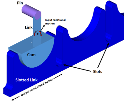
A slotted link mechanism. The cam is in contact with the slotted link as shown, whereas the pin comes into contact with the slots.
Step 1: Import CAD Geometry into MotionView.
| 1. | Copy the slotted_link.x_t file, located in the mbd_modeling\contacts folder, to your <working directory>. |
| 2. | Start a new MotionView session. |
| 3. | Click the the Tools menu, select Import CAD or FE…. |
Or
| - | Click on the Import Geometry icon  on the Standard toolbar. on the Standard toolbar. |
The Import CAD or FE dialog is displayed.
| 4. | Set the following options in this dialog: |
| - | Import Options radio button to Import CAD or Finite Element Model with Mass and Inertias. |
| - | Input File as Parasolid and specify the input CAD geometry as slotted_link.x_t in your <working directory> using the File Open icon . . |
| - | Notice the Output Graphic File text field is automatically populated with the same path and name, however it is suffixed with a _graphic.h3d extension. This is the file that will be used to specify the graphics in the model. You may change the name or path of the graphic H3D if you wish. |
| - | Expand the Meshing Options for Surface Data by clicking on the expand button ( ) if it is not already expanded. Ensure that the option to Allow HyperMesh to specify mesh options is checked. ) if it is not already expanded. Ensure that the option to Allow HyperMesh to specify mesh options is checked. |
| - | Activate the Control mesh coarseness for contacts check box. Set the slider to 5. This option tells HyperMesh to mesh the CAD geometry such that it can be used for 3D contact in MotionSolve. |
| Note | The slider controls the coarseness of the generated mesh, with 1 being the coarsest and 10 being the most fine. A very coarse mesh will have large triangles, which may not represent the curvature of the CAD surfaces accurately. Alternatively, a very fine mesh will have extremely small triangles that may increase element numbers and thereby the solution time. The best practice is to strike a balance between mesh fineness and performance that satisfies the modeling purpose. |
At this stage, the Import CAD or FE dialog should look like the figure below:
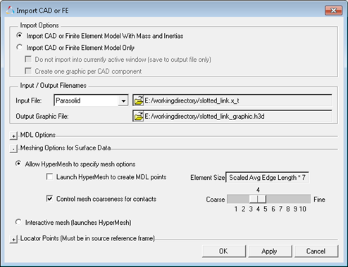
Importing CAD using the Import CAD or FE utility
MotionView will invoke HyperMesh in the background, to mesh the geometry and calculate its volume properties. Another dialog appears where the components in the CAD file can be reviewed along with their mass, density, and volume properties.
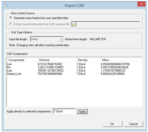
Importing CAD using the Import CAD or FE utility
| 6. | Click OK on this screen as well and Clear the Message Log. |
The converted geometry is loaded into MotionView for visual inspection. You can inspect the surface mesh by swapping the display to a meshed representation.
| 7. | Click on the Entity Attributes icon,  , on the Visualization toolbar. , on the Visualization toolbar. |
The Entity Attributes panel is displayed.
| 8. | Select all the graphics by clicking on Model at the top of the list at the left corner of the panel and click on Mesh Lines  . . |
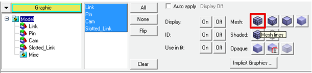
Displaying mesh lines for all the components of the input CAD geometry
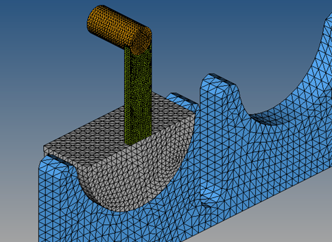
Displaying the surface mesh for all the components of the input CAD geometry
Step 2: Create Joints and Motion.
At this stage, the model contains the following bodies along with their associated graphics:
Entity name
|
Entity type
|
Description
|
Slotted_Link
|
Rigid Body
|
The slotted link body.
|
Cam
|
Rigid Body
|
The cam body.
|
Pin
|
Rigid Body
|
The pin body. Together the cam and the pin bodies engage the slotted link.
|
Link
|
Rigid Body
|
A connector body between the pin and the cam.
|
Slotted_Link
|
Graphic
|
The graphic that represents the slotted link body. This is a tessellated graphic.
|
Cam
|
Graphic
|
The graphic that represents the cam body. This is a tessellated graphic.
|
Pin
|
Graphic
|
The graphic that represents the pin body. This is a tessellated graphic.
|
Link
|
Graphic
|
The graphics that represent the link body. This is a tessellated graphic.
|
The Pin, Link, and the Cam bodies are fixed to each other and pivoted with to the Ground Body at the Cam center. The Slotted link can translate with respect to the Ground Body.
| 1. | Create joints  as per the details given in the table below: as per the details given in the table below: |
S.No
|
Label
|
Type
|
Body 1
|
Body 2
|
Origin
|
Alignment Axis
|
1
|
Pin Link Fix
|
Fixed Joint
|
Pin
|
Link
|
Pin CG
|
|
2
|
Link Cam Fix
|
Fixed Joint
|
Link
|
Cam
|
Link CG
|
|
3
|
Cam Pivot
|
Revolute Joint
|
Cam
|
Ground Body
|
Global Origin
|
Global Y
|
4
|
Sloted Link Slider
|
Translation Joint
|
Sloted_Link
|
Ground Body
|
Sloted_Link CG
|
Global X
|
| 2. | Apply a Motion  on the Cam Pivot joint of the type Displacement and the Expression as `360d*TIME`. on the Cam Pivot joint of the type Displacement and the Expression as `360d*TIME`. |
| 3. | Save  your model as slotted_link_mech.mdl. your model as slotted_link_mech.mdl. |
Step 3: Define contact between the colliding geometries.
In this step, you will define contact between:
| • | Cam and the Slotted_Link |
| • | Pin and the Slotted_Link |
| 1. | Right-click the  icon on the Force Entity toolbar. icon on the Force Entity toolbar. |
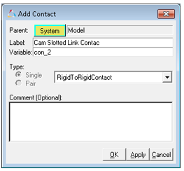
The Add Contact dialog is displayed.
| 2. | Change the Label to Cam Slotted Link Contact. Verify that RigidToRigidContact is selected and click OK. |
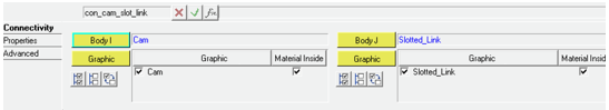
| 3. | From the Connectivity tab of the Contact panel, resolve Body I to Cam and Body J to Slotted_Link. Doing this will automatically select the respective graphics that are attached to these bodies. |
To make sure that the geometries are well defined, ensure that the normals are oriented correctly and there are no open edges or T-connections in the geometries.
| 4. | Activate the Highlight contact side check box. This will color the geometries specified for this contact force element according to the direction of the surface normals. Verify that both geometries are completely red, that is make sure that there are no blue patches for either geometry (to visualize clearly, you may have to deactivate the other graphic and reactivate). |
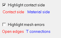
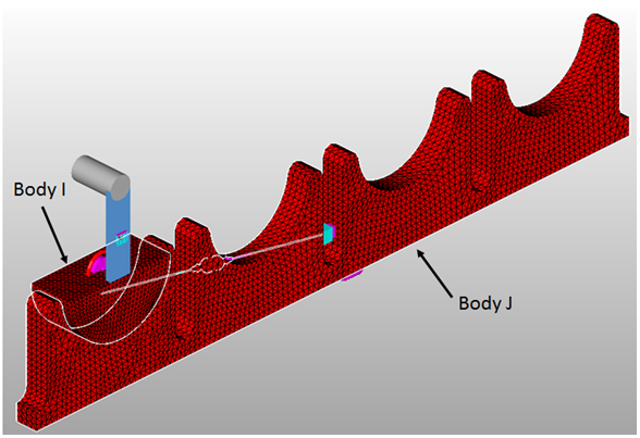
Checking for incorrect surface normals
The color red indicates the direction of surface normal and is the side of the expected contact.
Next, you can check for open edges or T-connections. If the associated graphics mesh has any open edges or T-connections, the Highlight mesh errors option would be active. If it is active, check the box for Highlight mesh errors. Doing this will highlight any open edges or T Connections in the geometry.
The graphics associated in this contact entity don’t have mesh errors. Hence you should see Highlight mesh errors grayed out.
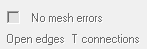
As you can see, the geometry seems to be clean and there are no free edges or T connections in the model.
| Note | For every Contact entity added to the model, MotionView automatically creates an Output  of the type Expression that can be used to plot the contact forces for that contact element. of the type Expression that can be used to plot the contact forces for that contact element. |
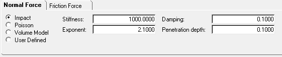
| 5. | Next, you need to specify the contact properties. Click on the Properties tab to bring up the Normal Force and the Friction Force property sub-tabs within the contact panel. In this model you will use an Impact model with the following properties: |
Normal Force Model
|
Impact
|
Stiffness
|
1000.0
|
Exponent
|
2.1
|
Damping
|
0.1
|
Penetration Depth
|
0.1
|
Friction Force Model
|
Disabled
|
Specify the properties as defined above in the contact panel.
| 6. | Repeat Steps 1 - 5 for creating contact between the Pin body (Body I) and the Slotted_Link (Body J). You may define the label for this contact to be Pin Slotted Link Contact. Define the same contact properties as listed in Step 5 above. |
| 7. | For the contact force element Pin Slotted Link Contact, you will also instruct MotionSolve to find the precise time at which contact first occurs between the two colliding bodies. Navigate to the Advanced tab. Check the box for Find precise contact event. In the text field below, specify a value of 0.01. |
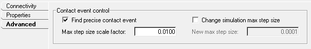
| Note | With the Find precise contact event option, MotionView automatically adds a sensor entity (defined by Sensor_Event in the solver deck), which has a “zero_crossing” attribute. During simulation, when the contact force is detected for the first time (force value crossing zero), MotionSolve will cut down its step size by the given factor and try to determine the contact event more precisely. |
Step 4: Setup a Transient Simulation and Run the Model.
At this point, you are ready to setup a transient analysis for this model.
| 1. | Navigate to the Run panel by clicking on the Run icon  on the toolbar. on the toolbar. |
| 2. | Change the Simulation type to Transient and specify an end time of 3.0 seconds. |
| 3. | To obtain accurate results, you will specify a smaller step size than the default. |
| - | Click on Simulation Settings…, to bring up the Simulation Settings dialog |
| - | Go to the Transient tab and set the Maximum Step Size to 1e-3. Click the Close button. |
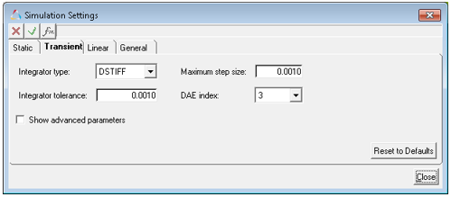
Specifying the Maximum Step Size
| 4. | From the Run panel, specify a name for your XML model and click on the Run button. The transient simulation is started. |
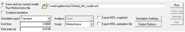
Specify the output file name and run the model
In the HyperWorks Solver View window that pops up, you should be able to see a message from the solver that confirms that the mesh based contact method is being used for the contact calculations.
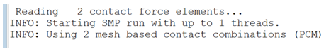
Verifying that the mesh based contact is used for the simulation
In the log file you will also see messages related to the sensor, this is related to finding the precise contact event for the second contact element in the model.
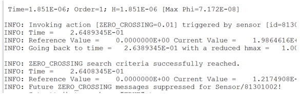
Solver message related to sensor activity
Step 5: Post-process the Results.
After the simulation is complete, MotionSolve prints out a summary table (both on screen and in the log file generated) that lists the top 5 contact pairs ordered by maximum penetration depth and by maximum contact force for this simulation. This is very useful since it can be used to verify that the model is behaving as intended even before loading the results (ABF, MRF, PLT or H3D) files. You can also use this table to verify that the penetration depths and contact forces are within the intended limits for your model. The summary table for this simulation is illustrated below:
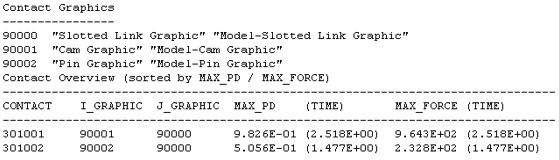
Contact Overview Table
| 1. | To view a consolidated report of the results, navigate to Assembly>View Reports. |
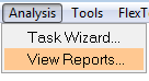
Analysis reports
This brings up a list of the history of simulations you have completed in the past using MotionView.
| 2. | Select the Contact Report that corresponds to this simulation. |
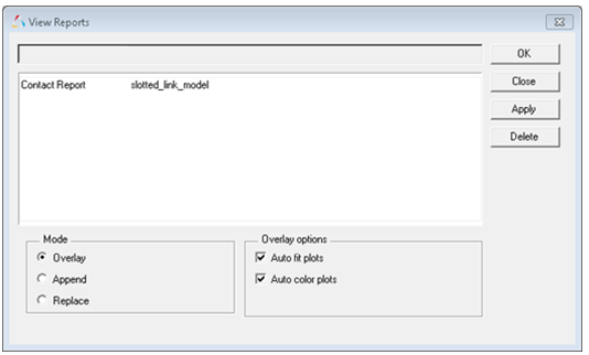
Create contact report
MotionView creates a number of pages in your current HyperWorks session:
| - | Contact Overview via H3D |
The first HyperView page (second in the session) displays a contour plot colored by maximum penetration depth over the entire length of the simulation. You may hide one or more parts to view this clearly in the graphic area. This is illustrated in the figure below. The cam graphic has been made transparent to see the penetration depths better.
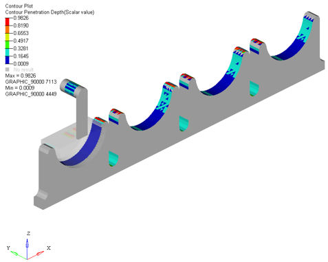
The contact overview for penetration depth
| Note | The contact overview colored by penetration depth is only available for meshed geometries. |
| - | Visualizing the penetration depth via H3D |
| • | Navigate to the next page  . . |
The third page in the session can be used to animate the results while viewing a contour plot of the penetration depth colored by magnitude. This allows you visualize the penetration depths at different times of the animation.
| • | Set the graphic display to Transparent Elements and Feature Lines. |
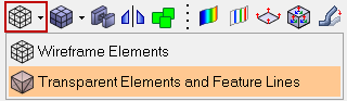
Setting all graphics display to transparent and feature lines
| • | Click on the Animation Controls icon,  , on the Animation toolbar and move the Animate End slider to the end , on the Animation toolbar and move the Animate End slider to the end  . . |
| • | Click on Contour panel button  on the toolbar and select the Cam body as the Components collector. on the toolbar and select the Cam body as the Components collector. |
| • | Click on the Start/Pause Animation button  to animate the result. to animate the result. |
The penetration depth contour animation on the cam body can be visualized.
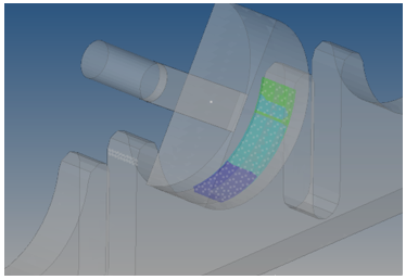
The contact penetration depth contour
| - | Visualizing the Contact forces via H3D |
| • | Navigate to the next page |
The fourth page in the session can be used to visualize the contact forces in the animation of the results. By default, the contact report plots the total contact force for each contact element.
| • | Click on the Animation Controls icon, , on the Animation toolbar and move the Animate End slider to the end . |
| • | Click on the Start/Pause Animation button to animate the result. |
| • | Set the graphic display to Transparent Elements and Feature Lines  . . |
| • | The forces may need to be scaled by magnitude or uniformly by a factor to be entirely visible. To change the scale, go to the Vector panel  , click on the Display tab and change the Size scaling option as appropriate. , click on the Display tab and change the Size scaling option as appropriate. |
An example of this animation is shown in the figure below:
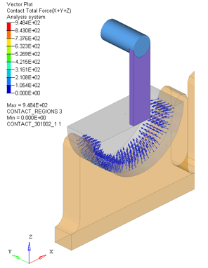
The total contact force between the cam body and the slotted link
The current force vectors are displayed on each node of the mesh that is in contact at each time step.
| - | Visualizing the sum total of force at a given region |
| • | From the Results browser deactivate the following Components: Contact Graphic(Cam Slotted Link Contact) and Contact Graphic (Pin Slotted Link Contact). Activate the Contact Region Output (by either clicking on the icon in the browser or using the right-click context menu). |
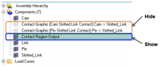
Deactivating and activating components from Results browser
MotionSolve supports a number of outputs that can be animated in HyperView:
| o | The contact normal force |
| o | The contact penetration depth |
| o | The contact penetration velocity |
| o | The contact point slip velocity |
| o | The contact tangential force |
| - | Visualizing MotionSolve outputs |
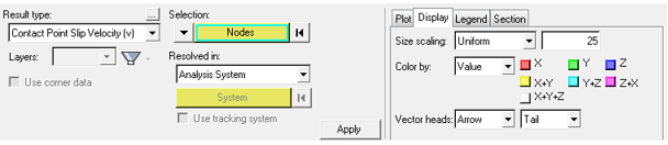
| • | Navigate to the Vector panel . |
| • | For the Result type, select the type of result you would like to see from the drop-down menu. Next, click Apply. |
This will plot the result type you selected for all the relevant graphics in the model. You may have to scale the force vectors accordingly to make sure they are visible.
Scaling the tangential force
As an example, the point slip velocity vectors are plotted in the figure below:
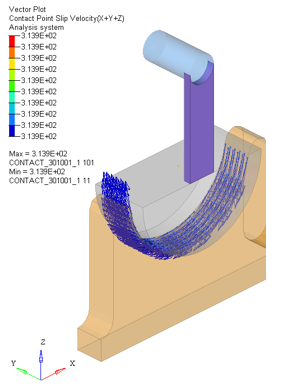
Point slip velocity vectors
| - | Plotting the contact forces via ABF |
| • | Navigate to the next page . This is the last page in the session. |
Each time a new contact entity is created in MotionView, a corresponding output force request is created that can be used to plot the contact forces between the graphics specified in the contact entity. These can then be visualized in HyperGraph. The last page of the contact report plots the contact force magnitude for all the contact elements in the model.
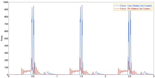
Total contact force magnitude
| - | Manually plotting other output requests |
| • | Click Add Page  and change the client to HyperGraph 2D and change the client to HyperGraph 2D  (if it is not already selected). (if it is not already selected). |
| • | Open  the ABF output file for the simulated model. the ABF output file for the simulated model. |
| • | Under Y Type, select Expressions and select a request in the Y Request window. |
As an example, select REQ/70000003 Force – Pin Slotted Link Contact as the Y Request and F4 as Y Component to plot.
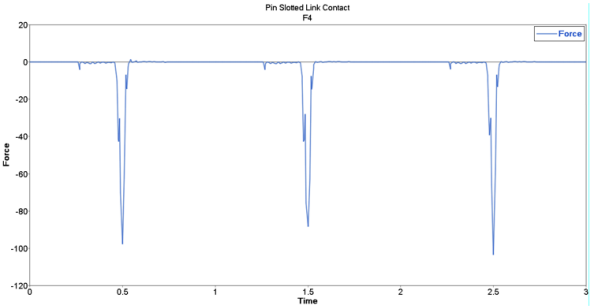
Visualizing the contact force in HyperGraph
| • | Save your session  as slotted_link.mvw. as slotted_link.mvw. |
Summary
In this tutorial, you learned how to create a good meshed representation from CAD geometry. Further, you learned how to setup contact between meshed geometries. Also, you were able to inspect the geometry to make sure the surface normals were correct and there were no open edges or T connections.
You were also able to setup a transient analysis to calculate the contact forces between these geometries and post-process the results via vector and contour plots in addition to plotting the contact force requests.


