In this tutorial, you will:
| • | Use Hyperstudy to set-up a DOE study of a MotionView model |
| • | Perform DOE study in the MotionView – HyperStudy environment |
| • | Create approximation (using the DOE results) which can be subsequently used to perform optimization of the MotionView model |
Theory
HyperStudy allows you to perform Design of Experiments (DOE), optimization, and stochastic studies in a CAE environment. The objective of a DOE, or Design of Experiments, study is to understand how changes to the parameters (design variables) of a model influence its performance (response).
After a DOE study is complete, approximation can be created from the results of the DOE study. The approximation is in the form of a polynomial equation of an output as a function of all input variables. This is called as the regression equation.
The regression equation can then be used to perform Optimization.
| Note | The goal of DOE is to develop an understanding of the behavior of the system, not to find an optimal, single solution. |
HyperStudy can be used to study different aspects of a design under various conditions, including non-linear behavior.
HyperStudy also does the following:
| • | Provides a variety of DOE study types, including user-defined |
| • | Facilitates multi-disciplinary DOE, optimization, and stochastic studies |
| • | Provides a variety of sampling techniques and distributions for stochastic studies |
| • | Parameterizes any solver input model via a user-friendly interface |
| • | Uses an extensive expression builder to perform mathematical operations |
| • | Uses a robust optimization engine |
| • | Includes built-in support for post-processing study results |
| • | Includes multiple results formats such as MVW, TXT for study results |
Tools
In MotionView, HyperStudy can be accessed from
| • | The Main-Menu under ‘Applications ->HyperStudy’ |
You can then select MDL property data as design variables in a DOE or an optimization exercise. Solver scripts registered in the MotionView Preferences file are available through the HyperStudy interface to conduct sequential solver runs for DOE or optimization.
For any study, the HyperStudy process is shown below:
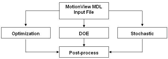
The HyperStudy process
MotionView MDL files can be directly loaded into HyperStudy. Any solver input file, such as ADAMS, MotionSolve, OptiStruct, Nastran, or Abaqus, can be parameterized and the template file submitted as input for HyperStudy. The parameterized file identifies the design variables to be changed during DOE, optimization, or stochastic studies. The solver runs are carried out accordingly and the results are then post-processed within HyperStudy.
Copy the files hs.mdl and target_toe.csv, located in the mbd_modeling\doe folder, to your <working directory>.
In the following steps, you will create a study to carry out subsequent DOE study on a front SLA suspension model.
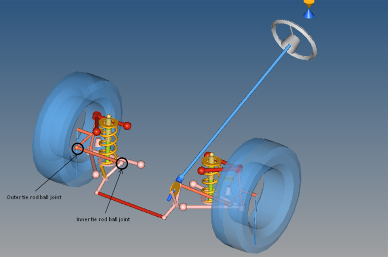
While performing a Static Ride Analysis, you will determine the effects of varying the coordinate positions of the origin points of the inner and outer tie-rod joints on the toe-curve.
Step 1: Study Set-up.
| 1. | Start a new MotionView session. |
| 2. | Click the Open Model icon,  , on the Model-Main toolbar. , on the Model-Main toolbar. |
Or
From the menu bar, select File > Open > Model.
| 3. | Select the file model hs.mdl, located in your <working directory>, and click Open. |
| 4. | Review the model and the toe-curve output request under Static Ride Analysis. |
| 5. | From the Applications menu, select HyperStudy. |
HyperStudy is launched. The message "Establishing connection between MotionView and Hyperstudy" is displayed.
| 6. | Start new study using one of the following ways: |
| - | From the Welcome page, click on the New Study icon,  . . |
Or
| - | From the toolbar, click the New Study icon, . |
Or
| - | From main menu, select File > New. The HyperStudy - Add Study dialog is displayed. |
Accept the default label and variable names.
Under Location, click the file browser and select <working directory>\.
| - | From the study Setup tree, select Define models. |
| - | Click  to open the Add Model dialog. to open the Add Model dialog. |
| - | Under Type, select MotionView to add a MotionView model to the study. |
| - | Accept the default variable name. |
| - | The following table with model data is created. |

Please note that following details are automatically filled when you define the model (previous step).
| o | Under Active, check the box to activate or deactivate the model from study. |
| o | The label of model entered in previous step. |
| o | The variable name of model entered in the previous step. |
| o | The model type selected in previous step. |
| o | Point to the source file (here model file is sourced from MotionView through the MotionView – HyperStudy interfacing). |
Enter a name for the solver input file with the proper extension (for Motionsolve ->.xml) and select the solver execution script MotionSolve - standalone ( ms ).
| 9. | Create design variables. |
| - | Click Import Variables to specify the design variables for the study. |
| - | The Model Browser window opens in MotionView, allowing you to select the variables interactively. |
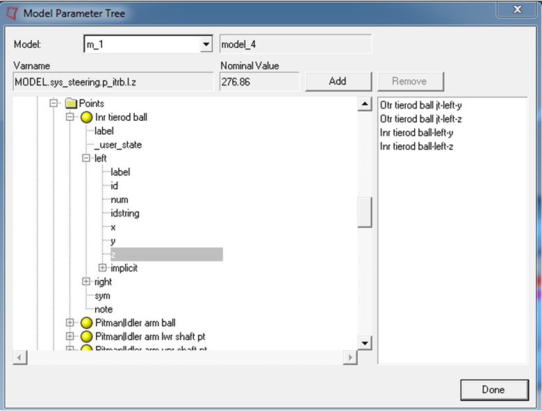
| - | Select the following from the Browser using the Model Parameter Tree dialog: |
System
|
Point
|
Coordinate
|
Function
|
Front SLA susp.
|
Otr tie-rod ball-jt -left
|
Y
|
Double-click or Click Add
|
Front SLA susp.
|
Otr tie-rod ball-jt –left
|
Z
|
Double-click or Click Add
|
Parallel Steering
|
Inr tie-rod ball - left
|
Y
|
Double-click or Click Add
|
Parallel Steering
|
Inr tie-rod ball - left
|
Z
|
Double-click or Click Add
|
Model Parameter Tree dialog
| - | Click Next to go to Define Design Variables. |
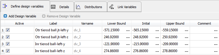
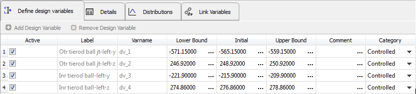
| 10. | Define design variables. |
| - | From the Define design variables tab, edit the upper and lower bounds of the design variables according to the following table. |
Point
|
Coordinate
|
Lower
|
Upper
|
Outer tie-rod ball-jt -left
|
Y
|
-571.15
|
-559.15
|
Outer tie-rod ball-jt - left
|
Z
|
246.92
|
250.92
|
Inner tie-rod ball - left
|
Y
|
-221.9
|
-209.9
|
Inner tie-rod ball - left
|
Z
|
274.86
|
278.86
|
| - | This step also includes definition of other properties to the design variables. The options Details and Distributions specify variations of design variables in the range specified. The option Link Variables is used to link different design variables through a mathematical expression. |
| - | Click on each tab to observe these options. |
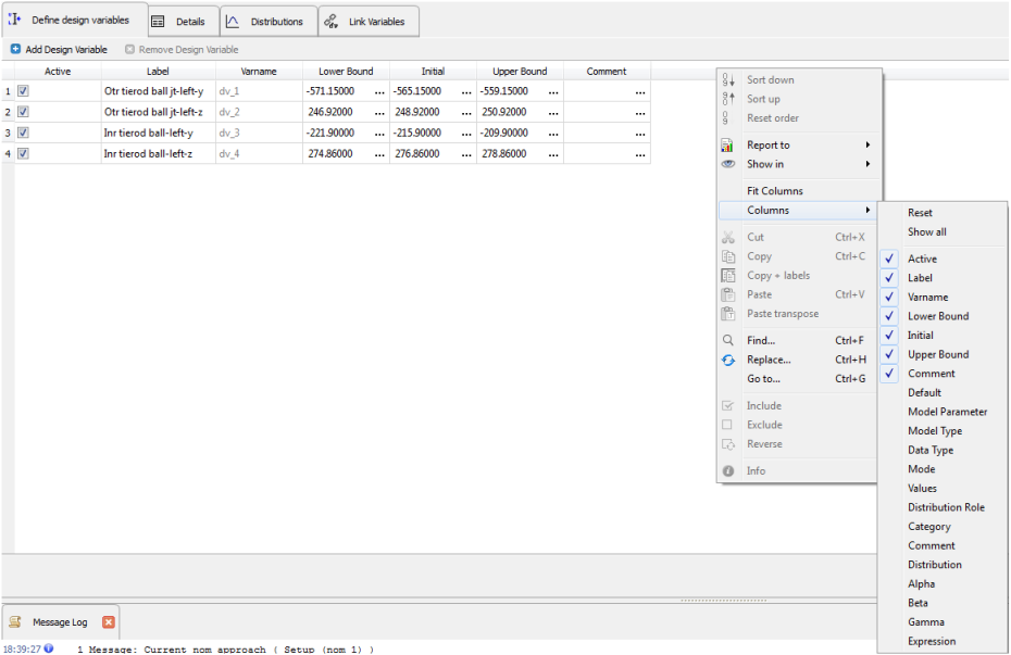
| - | Right click on the column header row to view more options that you may want to add. |
- Click Next to go to Specifications.
This section allows you to specify the initial run for DOE.
| - | Select the Nominal Run radio button for this study and click the Apply button. |
| - | Click Next to go to Evaluate. |
| - | Click Evaluate Tasks to perform the nominal run. |
| - | Make sure that all settings for the run (Write, Execute and Extract) are activated. |
MotionSolve runs in the background and the analysis is carried out for the base configuration. Please note the messages in status bar of the HyperStudy interface and the MotionView interface. If message log is not visible, click the Message log button,  , or go to View > Message log to display the log.
| - | Once the nominal run is complete, click Next to go to Define responses. |
| - | Click Add Response to add a new response. |
| - | Label the response Sum of Squared Error. |
| - | Accept the variable name and click OK. |
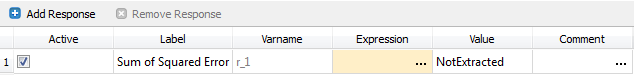
Response table data
| - | Click the ellipses, …, in the Expression cell of Response table to launch the Expression Builder. |
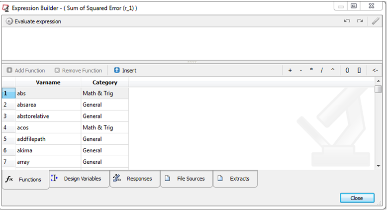
Expression builder
Note: You can move the cursor over the function to display the function help.
For this exercise, the response function requires two vectors:
| - | The elements of Vector 1 contain actual data points of the toe curve from the solver run for the nominal configuration. |
| - | The elements of Vector 2 contain data points from the target curve. |
| - | Click the File Sources tab to source the data from the files. |
Vector 1:
| - | Click  to display the HyperStudy - Add dialog box. to display the HyperStudy - Add dialog box. |
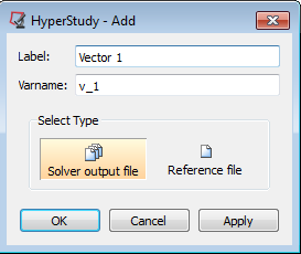
| - | Accept the default label and variable name. |
| - | For Select Type, select Solver output file. |

Response data table
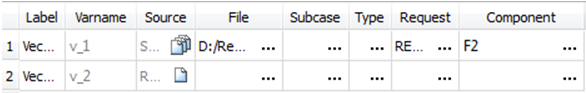
| - | Click the ellipses, …, in the File cell of vector table data to launch the Vector Source – (Vector 1(v_1)) dialog box. |
| - | Click the file browser button,  , and select the file m_1.mrf from <working directory>\approaches\nom_1\run__00001\m_1\. , and select the file m_1.mrf from <working directory>\approaches\nom_1\run__00001\m_1\. |
| - | This enables the Type, Request and Component fields. |
| - | From the Type drop-down menu, select Expressions. |
| - | From the Request drop-down menu, select REQ/70000033 toe-curve. |
| - | From the Component drop-down menu, select F2. |
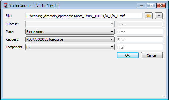
Vector 1 source dialog box
You have now selected the toe curve data from the solver run as the data elements for Vector 1.
| - | Click on the arrow button,  , on the right side of the dialog box to expanding the vector dialog box and preview the curve. , on the right side of the dialog box to expanding the vector dialog box and preview the curve. |
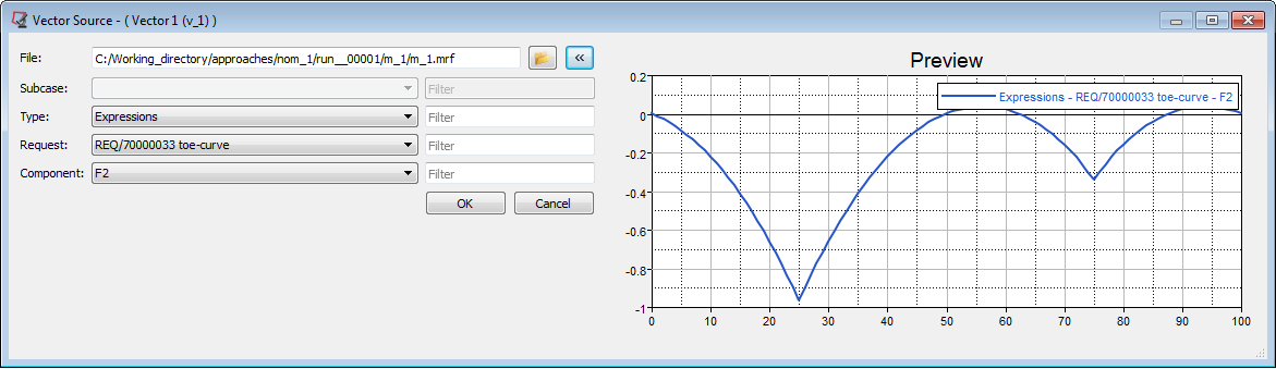
Expanded dialog box of Vector 1 source
Vector 2:
Create a vector to hold the data elements from the target toe curve.
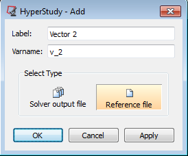
| - | Click Add File Source to display the HyperStudy - Add File Source dialog box. |
| - | Accept the default label and variable name. |
| - | For Select Type, select Reference file. |
Response data table
| - | Click the … in the File cell of the Vector 2 table data to launch the Vector Source – (Vector 2(v_2)) dialog box. |
| - | Click the file browser button, , and select the file target_toe.csv, located in your <working directory>\. |
| - | Set Type to Unknown and Request to Block 1. |
| - | From the Component drop-down menu, select Column 1. |
| 14. | In the Expression field, create the following expression: |
sum((v_1-v_2)^2)
This expression evaluates the sum of the square of the difference between the “actual toe change” values (from solver run) and the “targeted toe curve” (from imported file). In the next tutorial, MV-3010, we will use HyperStudy to minimize the value of this expression to get the required suspension configuration.
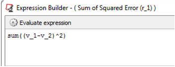
| 15. | Click Evaluate expression to verify that the expression is evaluated correctly. You should get a value of 16.289. |
| - | If you do not encounter any error messages and were able to successfully extract the response for the nominal run, click Next to go to Post Processing. |
| - | Observe the table with the design variable values used for the nominal run and other tabs with the post-processing options. |
| - | Click Next to go to Report. |
| - | Observe various reporting formats available. The images and data captured during the post-processing can be exported in any of the formats provided on Report page. |
| 16. | From the File menu, select Save As…. |
| 17. | Save this study set-up as Setup.xml to your <working directory>\. |
Step 2: DOE Study.
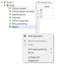
| - | Right-click in the Explorer browser area and from the context menu, click  Add Approach… to display the Add Approach dialog. Add Approach… to display the Add Approach dialog. |
Or
| - | From the Edit menu bar, click the Add Approach option to display the HyperStudy - Add dialog. |
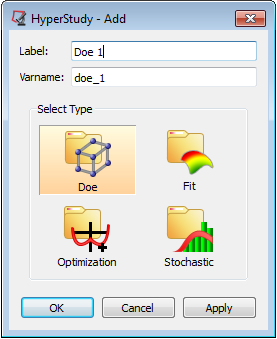
| - | Under Select Type, select Doe. |
| - | Accept the default label and variable name and click OK. |
The DOE study tree is displayed in the Browser with name Doe 1.
| - | Click Next to go to Select design variables. |
| 2. | Select design variables for the DOE study. |
| - | All variables are used in the present DOE study, so make sure that all design variables are active. |
| - | All the design variables in this study are controlled. Therefore, for Category, leave all variables set to Controlled. |
| - | Click Next to go to Select responses. |
| 3. | Select responses for the DOE study: |
| - | There is only one response in the present study - make sure to select the response. |
| - | Click Next to go to Specifications. |
| 4. | Specifications for the DOE study: |
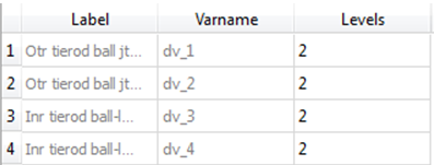
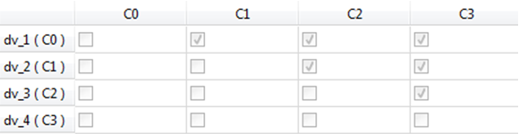
The design space for the DOE study is created in this step. The present study has four design variables with two levels each. A full factorial will give 24 = 16 experiments, as the number of experiments are less. We will do a full factorial run. Selecting any mode from the list shows all possible options in the Parameters panel area on the left side of GUI.
| - | Click the Levels tab to see the design variables and number of levels. |
| - | Click the Interaction tab to observe that all interactions are selected as it is a full factorial run. |
Note: Options which are not applicable will be grayed out or a message will be shown.
5. Click Apply to generate the design space.
6. Click Next to go to Evaluate.
DOE run:
| The Tasks tab of Evaluate shows a table of 16 rows and four columns. Column 1 shows the experiment number while other columns corresponding to each experiment get updated with the experiment status of failure or success in the three stages of model execution: Write, Execute and Extract. |
| Design variable values used under each experiment can be seen under the Evolution Data tab. |
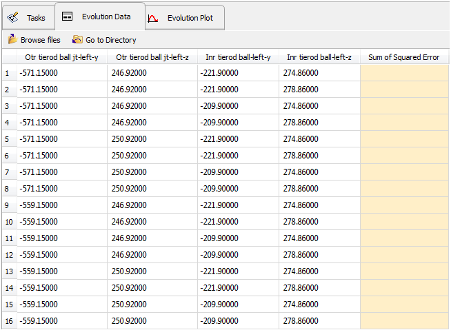
The last column corresponds to the response value from each run. The values gets populated once the run is completed.
| - | Click Evaluate Tasks to start the DOE study. |
| Once all the runs are finished, the tasks table gets filled up with the status for each run (Success/Fail). |
| - | In the present DOE study, all runs are successfully completed. Click Next to go to Post Processing. |
7. Viewing Main Effect and Interaction plots:
The post-processing section has variety of utilities to helps user to effectively post process results. Run Summary tab of Post processing page will provide a summary of design along with responses.
The New Generation HyperStudy allows you to sort data by right-clicking on the column heading and selecting the options from context menu.
The options to post-process are available in other tabs. The main effects can be plotted by selecting the Linear Effects tab.
Main Effects:
| - | Click the Linear Effects tab to open the main effects plot window. From the Channel page, select Variables and Responses for which main effects need to be plotted. Press the left mouse button and move over the variable or responses list for multiple selection. |
| - | Select all controlled variables and responses to plot the main effect plot. This plot shows the effect of each parameter on the response. |
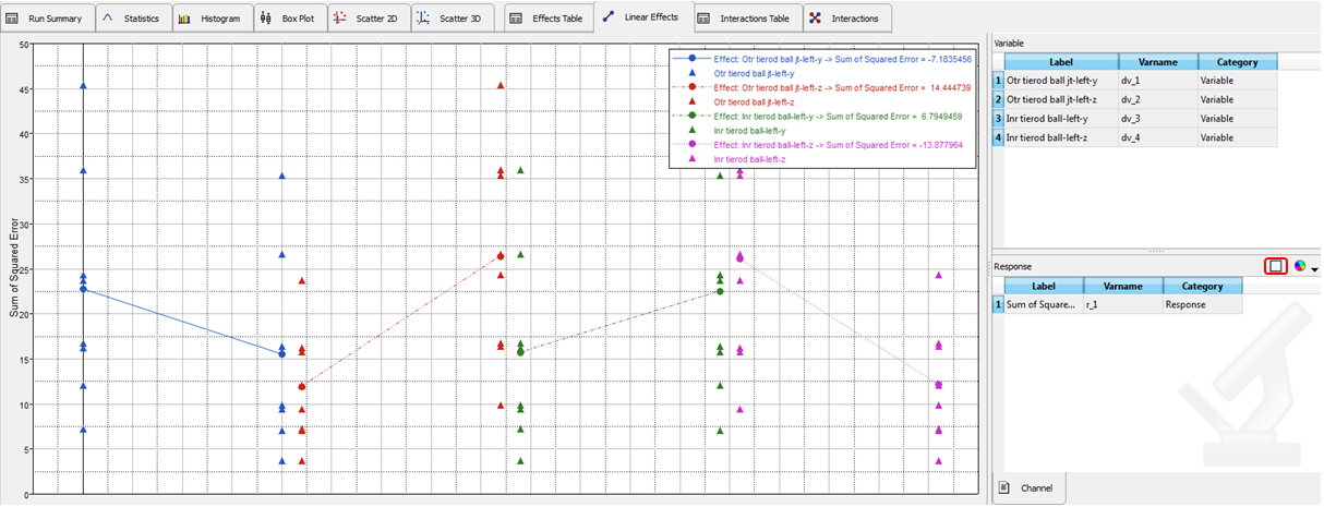
DOE – Main effects plot
Note: Click on window icon,  , (highlighted above) to toggle it to multiple windows,
  . Each curve is displayed in a different plot window.
Interactions:
Interactions can be plotted from the Interactions tab following the above procedure. Here, we will use the post-processing window to plot the interactions. Click Launch Post Processing to display the Post-processing window.
Display the Regressions in one of the following ways:
| - | From the toolbar, click the Display regressions icon,  . . |
Or
| - | From main menu, select Display > Regressions. |
| - | Click the Interactions radio button. |
By default, all interactions are displayed.
| - | Click View to select the design variables Otr_tierod_ball_jt-left-z and Inr_tierod_ball_jt-left-z. |
| - | Under Display on the left side of the page, change the variables type from All Variables to Controlled Variables from the drop-down menu next to View button. This displays the interaction plot for these two variables only. |
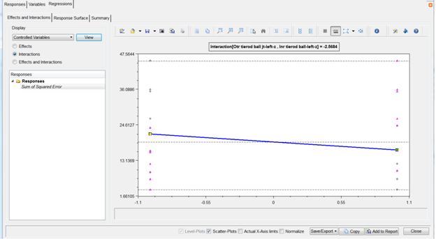
Controlled design variable plot for “Otr_tierod_ball_jt-left-z” & “Inr_tierod_ball_jt-left-z” interaction
| - | Close the Post Processing application. Confirm the request to quit the application. |
Step 3: Approximation.
System response is approximated by using various curve fitting methods. An approximation for the response with the design variables variation is calculated using the data from above DOE study. The accuracy of the approximation can be checked and improved.
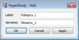
1. Adding an approximation.
| - | Right-click in the Browser area and from the context menu, click Add Approach to display the Add Approach dialog. |
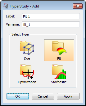
| - | Under Select Type, select Fit. |
| - | Accept the default label and variable names and click OK. |
| - | A new tree with the name Fit 1 is created in the Browser. |
2. Input matrix.
| - | Click  to display the HyperStudy - Add dialog. to display the HyperStudy - Add dialog. |
| - | Accept the default label and variable names. |
A matrix table is created. Select the following options to specify the DOE results as the input matrix.
| - | Under Type, use the drop-down menu to select Input. |
| - | For Matrix Source, select Doe 1 from the drop-down menu. |
In the present study, we are not using any validation matrix. So, no matrix will be added for validation matrix.

Observe that the status shows “Import pending”.
| - | Click Import Matrix to import the DOE results for the input matrix. |
| - | Click Next to go to Select design variables. |
| - | Select all design variables and click Next to go to Select responses. |
| - | Select the response and click Next to go to Specifications. |
In this section, the approximation type and it’s properties are defined.
Select Moving Least Squares (SMLS):
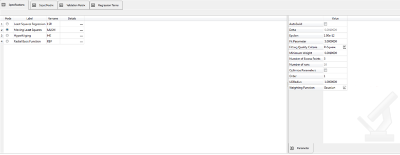
| - | Click Apply to apply the approximation method. |
| - | Click Next to go to Evaluate. |
| - | Observe an empty Tasks table which corresponds to the DOE experiments. |
| - | Click Evaluate Tasks to evaluate the approximation for the DOE experiments. |
Upon completion, the table is populated with the status value (Success or Fail).
| - | Click the other tabs available to observe the fit. |
| - | Click the Evolution Data tab to observe the experiment table with responses from the MotionSolve run and responses predicted using approximation. The same can be viewed in graph format by selecting the Evolution plot tab. |
| - | Select Sum of Squared of Squared Error and Squared of Squared Error_MLSM to plot against the experiment numbers. |
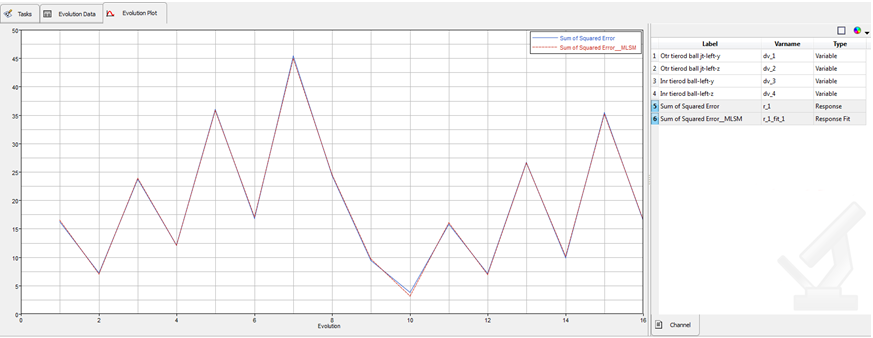
This fit shows a good approximation to the response.
| - | Click Next to go to Post Processing. |
| - | Post-processing provides you with statistical parameters and graphical tools useful in validating the correctness of approximation. |
| - | The Residuals tab shows the difference between the response value from the solver and the response value from the regression equation. |
| - | The residual values can be used to determine which runs are generating more errors in the regression model. |
| - | The Trade-off 3D tab shows the plots of the main effects vs. response from the approximation. |
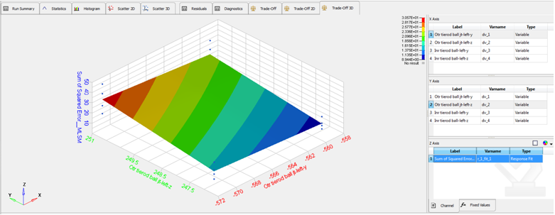
Trade-off: 3-D plots
| - | From the toolbar, click the Save icon,  , to save the study. , to save the study. |
| Note | All study files will be saved in the study directory with the folder names that are the same as the tree varnames. For example, nom_1,doe_1 and fit_1. |


