MV-7000: Modeling Differential Equations Using MotionView and MotionSolve

Differential equations are very versatile and have many different applications in modeling multi-body systems. User-defined dynamic states are commonly used to create low pass filters, apply time lags to signals, model simple feedback loops, and integrate signals. The signal may be used to:

•	define forces.

•	used as independent variables for interpolating through splines or curves.

•	used as input signals for generic control modeling elements.

•	define program output signals.

The MotionSolve expressions and user-subroutines allow you to define fairly complex user-defined dynamic states.

The expression type is used when the algorithm defining the differential equation is simple enough to be expressed as a simple formula. In many situations, the dynamic state is governed by substantial logic and data manipulation. In such cases, it is preferable to use a programming language to define the value of a differential equation. The user-defined subroutine, DIFSUB, allows you to accomplish this.

Step 1: Build and analyze a simplified model.

In the following exercise, we will build and analyze a simplified model of a pressure vessel blown down using MotionView and MotionSolve.

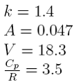
1.	We specify the following parameters (state variables) as solver variables:

mv7000_eq1

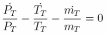
2.	Model the following differential equations:

mv7000_eq2

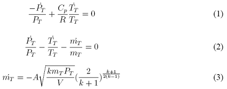
The three states of the system are PT ,TT and mT.

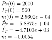
3.	Specify the initial conditions for the system as:

mv7000_eq3

4.	Run the model in MotionSolve and post-process the results in HyperGraph.

Creating Solver Variables

A solver variable defines an explicit, algebraic state in MotionSolve. The algebraic state may be a function of the state of the system or any other solver variables that are defined. Recursive or implicit definitions are not allowed at this time.

Two types of solver variables are available. The first, and probably the most convenient, is the expression valued variable. The second is the user-subroutine valued variable.

The expression method is used when the algorithm defining the algebraic state is simple. In many situations, the algebraic state is governed by substantial logic and data manipulation. In those cases, it is preferable to use a programming language to define the value of a solver variable. The user-defined subroutine, VARSUB, enables you to do this.

Solver Variables are quite versatile and have many different applications in modeling multi-body systems. They are commonly used to create signals of interest in the simulation. The signal may then be used to define forces, independent variables for interpolation, inputs to generic control elements, and output signals.

MotionSolve expressions and user-subroutines allow for fairly complex algebraic states to be defined.

For more information, please refer to the MotionView and MotionSolve User's Guides in the on-line help.

Step 2: Add a solver variable.

1.	Launch a new session of MotionView.

2.	From the Project Browser, right-click on Model and select Add > Control Entity > Solver Variable (or right-click on the Solver Variables icon,, from the toolbar).

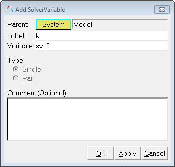
3.	The Add Solver Variable dialog is displayed.

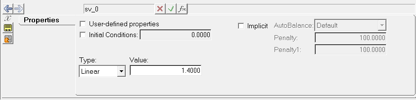
4.	In the Label field, assign the label K to the solver variable.

5.	In the Variable field, assign a variable name to the solver variable or leave the default name.

Click OK.

mv7000_addsolvar

7.	From the Properties tab, under Type:, select Linear and enter a value of 1.4 in the field.

mv7000_solvarpanel2

8.	Repeat steps 1 through 7 to create the three remaining solver variables:

mv7000eq4

Step 3: Modeling differential equations.

1.	From the Project Browser, right-click on Model and select Add General MDL Entity > Solver Differential Equation (or right-click on the Solver Differential Equation icon, , from the toolbar.

2.	The Add SolverDiff dialog is displayed.

3.	In the Label field, assign a label to the solver diff or leave the default label.

4.	In the Variable field, assign a variable name to the solver diff or leave the default name.

5.	Click Apply twice.

6.	Click OK. Now, three solver differential equations will be created.

7.	Next, we'll model the first differential equation:

mv7000eq5

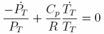
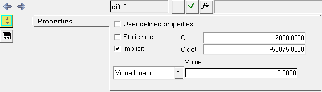
This is an implicit differential equation that has a constant (Cp/R). The initial condition of the differential equation (IC) and its first derivative (IC dot) are known (given).

8.	Select SolverDiff 0. From the Properties tab, select Implicit and specify IC and IC dot as 2000 and -58875, respectively.

mv7000_solvarpanel3

9.	Select the type as Expression.

10.

To access the expression builder, click in the text field and select the F(x) button,

, from the trio of buttons at the top of the panel,

. This will display the Expression Builder. In this dialog, you can enter expressions in text boxes without extensive typing and memorization. It can be used to construct mathematical expressions.

11.	Populate the expression as shown in the image below:

mv7000exprbldr

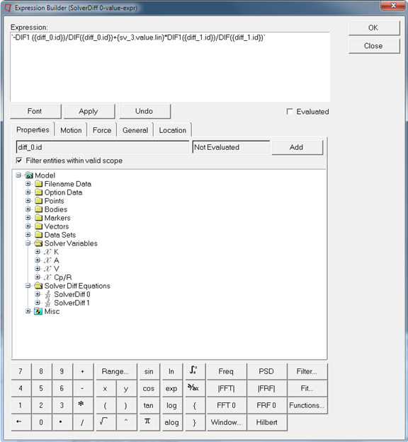
`-DIF1 ({diff_0.id})/DIF({diff_0.id})+{sv_3.value.lin}*DIF1({diff_1.id})/DIF({diff_1.id})`

You can use the model tree to access entity variables in your model. As you can see for the above expression, to refer to the ID of the differential equation, browse for it from the list-tree on the Properties tab and select the ID. Click Apply. The name of the selected entity or property is inserted into the expression.

12.	Click OK. The new expression is displayed in the text box on the panel.

13.	Repeat steps 8 through 13 to modify the remaining two differential equations:

mv7000_eq6

Implicit: Yes.

IC: 560

IC_dot: -4710

Value Expression:

`DIF1({diff_0.id})/DIF({diff_0.id})-DIF1({diff_1.id})/DIF({diff_1.id})-DIF1({diff_2.id})/DIF({diff_2.id})`

mv7000_eq7

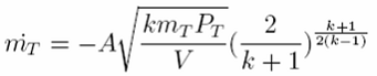
Implicit: No.

IC: 0.000256

Value Expression:

`-{sv_1.value.lin} *sqrt({sv_0.value.lin}*DIF({diff_2.id})*DIF({diff_0.id}) /{sv_2.value.lin})*0.5787`

Step 4: Running the model in MotionSolve.

1.	Click the Run button, , on the toolbar. The Run panel is displayed.

2.	Specify the values as shown below:

mv7000simparam

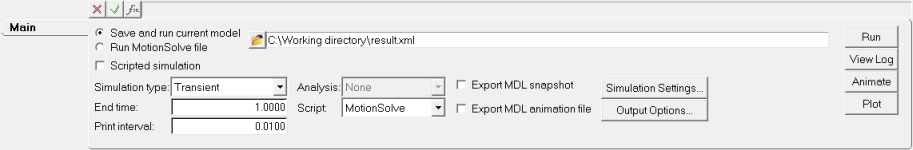
3.	Under the Main tab, choose the Save and run current model radio button.

4.	Click on the browser icon, , specify a filename of your choice.

5.	Click Save.

6.	Click Check Model button, , to check the model.

7.	To run the model, click Run. The solver will get invoked here.

8.	Post-process the results using Altair HyperGraph.