MV-1029: Modeling Point-to-Deformable-Surface Force (PTdSF)

In this tutorial, you will learn how to:

•	Model a PTdSFforce (point-to-deformable-surface) joint with a contact force

A PTdSFforce (point-to-deformable-surface) joint is a higher pair constraint with an added contact force. The force is either modeled as a linear one or a Poisson type here. This constraint restricts a specified point on a body to move along a specified deformable surface on another body. The point may belong to a rigid, flexible or point body. The deformable surface for this tutorial is defined on a rigidly supported plate. A mass is constrained to move on the surface with a PTdSFforce constraint. The added feature here is that a flexible contact force acts at the center of mass of the ball between it and the deformable surface. In this tutorial we will take up the case of the linear force model.

Exercise

Copy the following files Plate.h3d and membrane.fem, located in the mbd_modeling\interactive folder, to your <working directory>.

Step 1: Creating points.

Let’s start with creating points that will help us locate the bodies and joints as required. We will define points for center of mass of the bodies and joint locations.

1.	Start a new MotionView Session. We will work with the default units (kg, mm, s, N).

2.	From the Project Browser right-click on Model and select Add Reference Entity > Point (or right-click the Points icon on the Model-Reference toolbar).

The Add Point or PointPair dialog is displayed.

3.	For Label, enter BallCM.

4.	Accept the default variable name and click OK.

5.	Click on the Properties tab and specify the coordinates as X = 0.0, Y = 0.0, and Z = 50.0.

6.	Follow the same procedure for the other points specified in the following table:

Point	X	Y
PointMembInterface39	-55.00	-55.00
PointMembInterface40	55.00	-55.00
PointMembInterface41	55.00	55.00
PointMembInterface42	-55.00	55.00

Step 2: Creating Bodies.

We will have two bodies apart from the ground body in our model visualization: the membrane and the ball. Pre-specified inertia properties will be used to define the ball.

1.	From the Project Browser right-click on Model and select Add Reference Entity > Body (or right-click the Body icon on the Model-Reference toolbar).

The Add Body or BodyPair dialog is displayed.

2.	For Label, enter Membrane and click OK.

3.	Accept the default variable name and click OK.

For the remainder of this tutorial - accept the default names that are provided for the rest of the variables that you will be asked for.

4.	From the Properties tab, check the Deformable box.

5.	Click on the Graphic file browser icon and select Plate.h3d from the <working directory>.

The same path will automatically appear next to the H3D file browser icon .

6.	Right-click on Bodies in the Project Browser and select Add Body.

The Add Body or BodyPair dialog is displayed.

7.	For Label, enter Ball and click OK.

8.	From the Properties tab, specify the following for the Ball:

Body	Mass	Ixx	Iyy	Izz	Ixy	Iyz	Izx
Ball	1.00	40000.00	40000.00	40000.00	0.0	0.0	0.0

9.	For the Ball body, under the CM Coordinates tab, check the Use center of mass coordinate system box.

10.	Double click on Point.

The Select a Point dialog is displayed.

11.	Choose BallCM and click OK.

12.	Accept defaults for axes orientation properties.

Step 3: Creating Markers and a Deformable Surface.

Now, we will define some markers required for the membrane.

1.	From the Macros menu, select Create Markers For Deformable Surface.

mv-1028_crte_mrkrs_macro

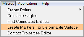
The Create Markers For a Deformable Surface utility is displayed at the bottom of the screen.

2.	For Select the Body, use the Body input collector to select Membrane.

mv-1028_crte_mrkrs_macro_panel

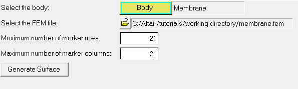
3.	Click on the Select the FEM file file browser icon and select the membrane.fem file.

4.	Use the default values for the Maximum number of marker rows and Maximum number of marker columns.

5.	Click Generate.

The Markers and Deformable Surface are created.

Step 4: Creating Joints.

Here, we will define all the necessary joints. We require four joints for the model, all of them being fixed joints between the membrane and the ground.

1.	From the Project Browser right-click on Model and select Add Constraint > Joint (or right-click the Joints icon on the Model-Constraint toolbar).

The Add Joint or JointPair dialog is displayed.

2.	For Label, enter Joint 1.

3.	Select Fixed Joint as the type and click OK.

4.	From the Connectivity tab, double-click on Body 1.

The Select a Body dialog is displayed.

5.	Choose Membrane and click OK.

6.	From the Connectivity tab, double-click on Body 2.

The Select a Body dialog is displayed.

7.	Choose Ground Body and click OK.

8.	From the Connectivity tab, double-click on Point.

The Select a Point dialog is displayed.

9.	Choose PointMembInterface39 and click OK.

10.	Repeat the same procedure for the other three joints.

A table is provided below for your convenience:

Label	Type of Joint	Body 1	Body 2	Point
Joint 2	Fixed	Membrane	Ground Body	PointMembInterface40
Joint 3	Fixed	Membrane	Ground Body	PointMembInterface41
Joint 4	Fixed	Membrane	Ground Body	PointMembInterface42

Step 5: Creating Contacts.

Here we will define the contact force between the deformable membrane and the ball.

1.	From the Project Browser right-click on Model and select Add Force Entity > Contact (or right-click the Contacts icon on the Model-Force toolbar).

The Add Contact dialog is displayed.

2.	For Label, enter Contact 0.

3.	Select PointToDeformableSurfaceContact for the type of contact and click OK.

4.	From the Connectivity tab; select Linear as the calculation method, Ball for Body, BallCM for Point, and DeformableSurface 1 for DeformableSurface.

5.	Uncheck the Flip normal checkbox.

6.	Click on the Properties tab and enter 10 for Radius, 1000 for Stiffness, and 0.2 for Damping.

Step 6: Creating Graphics.

Graphics for the ball will now be built here.

1.	From the Project Browser right-click on Model and select Add Reference Entity > Graphic (or right-click the Graphics icon on the Model-Reference toolbar).

The Add Graphics or GraphicPair dialog is displayed.

2.	For Label, enter Ball.

3.	For Type, choose Sphere from the drop-down menu and click OK.

4.	From the Connectivity tab, double-click on Body.

The Select a Body dialog is displayed.

5.	Choose Ball and click OK.

6.	Again from the Connectivity tab, double-click on Point.

The Select a Point dialog is displayed.

7.	Choose BallCM and click OK.

8.	From the Properties tab, enter 10 as the radius of the Ball.

9.	From the Visualization tab, select a color for the Ball.

Step 7: Return to the Bodies Panel.

1.	Click the Body icon on the Model-Reference toolbar.

2.	For the membrane which has already been defined, click on the Nodes button.

The Nodes dialog is displayed.

3.	Uncheck the Only search interface nodes box and then click on Find All.

4.	Close the the Nodes dialog.

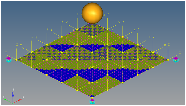
At the end of these steps your model should look like the one shown in the figure below:

mv-1029_pic7

Step 8: Running the Model.

Now we have the model defined completely and it is ready to run.

1.	Click the Run icon on the Model-Main toolbar.

The Run panel gets displayed.

2.	From the Main tab, specify values as shown below:

mv-1029_pic2

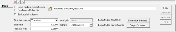
3.	Choose the Save and run current model radio button.

4.	Click on the browser icon and save the file as result.xml in the <working directory>.

5.	Click Save.

6.	Click the Check Model button on the Model Check toolbar to check the model for errors.

7.	To run the model, click the Run button on the panel.

The solver will get invoked here.

Step 9: Viewing the Results.

1.	Once the solver has finished its job, the Animate button will be active. Click on Animate.

The can be used to start the animation, and the icon can be used to stop/pause the animation.

One would also like to inspect the displacement profile of the membrane and the ball. For this, we will plot the Z position of the center of mass of the ball.

2.	Click on the Add Page icon and add a new page.

3.	Use the Select application drop-down menu to change the application from MotionView to HyperGraph 2D .

4.	Click the Build Plots icon on the Curves toolbar.

5.	Click on the browser icon and load the result.abf file from the <working directory>.

6.	Make selections for the plot as shown below:

mv-1029_pic3

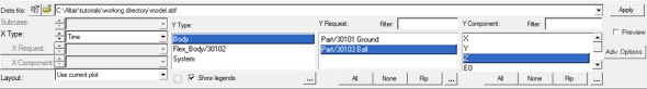
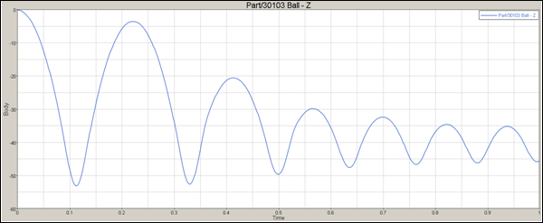
We are plotting the Z position of the center of mass of the ball.

7.	Click Apply.

The profile for the Z-displacement of the ball should look like the one shown below:

mv-1029_pic8

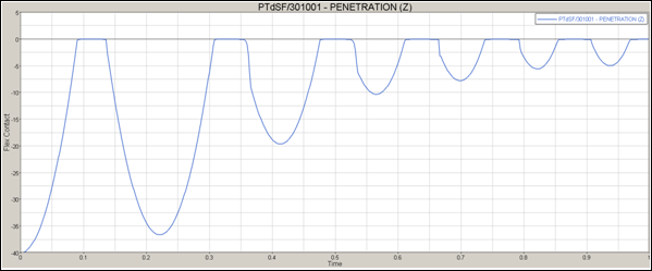
We can also plot the penetration distance for this flexible contact.

1.	Make selections for the plot as shown below:

mv-1029_pic5

2.	Click Apply.

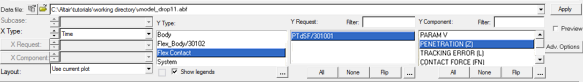
3.	The penetration profile as a function of time looks like the one shown below:

mv-1029_pic6