In this tutorial you will learn how to:
| • | Use Spline3D to model an input which depends on two independent variables. |
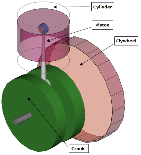
This will be accomplished by building a Single Cylinder Engine model similar to the one shown below:
What are Spline3Ds?
Spline3Ds are reference data plotted in three-dimensional coordinates which have two independent vectors or axis. These can be visualized as a number of 2D Splines (Curves) placed at regular intervals along a third axis. For instance, a bushing is generally characterized by a Force versus the Displacement curve. Let’s say, the Force versus displacement also varies with temperature. Effectively, there are two independent variables for the bushing force - Displacement and Temperature. Another example is the Engine Pressure (or Force) versus the Crank angle map (popularly known as P-Theta diagram). The P-theta map will vary at different engine speeds (or RPM). Such a scenario can be modeled using Spline3D.
Exercise
In this exercise, an engine mechanism is simulated where the combustion force that varies with regard to the crank angle and engine speed is modeled using Spline3D.
Step 1: Reviewing the model.
| 1. | Copy the files SingleCylEngine.mdl and FTheta.csv , located in the mbd_modeling\interactive\spline3d folder, to your <working directory>. |
| 2. | Start a new MotionView session. |
| 3. | Open the SingleCylEngine.mdl model file. |
| - | The model is a piston cylinder mechanism with a flywheel. |
| - | The model has two systems: System Cyl1 and System Flywheel. |
| - | In the System Flywheel, the Flywheel (fixed to Crank) is driven by a velocity based Motion between markers which refers to a curve (Crank_RPM) for inputs. |
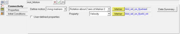
Motion Panel - Connectivity Tab
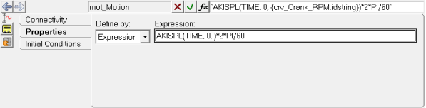
Motion Panel - Properties Tab (with Expression referring to the Curve using AKISPL function)
| - | The curve Crank_RPM indicates the time history of crank speed during the simulation. The speed ramps up to 500 RPM and then to 1000, 1500, and 2000 RPM. |
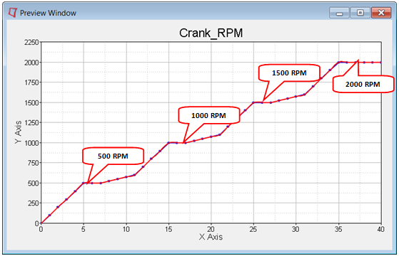
Curve Crank_RPM
| - | Two Solver Variables: Crank_angle (deg) and Crank_RPM keep track of the angular rotation (in degrees) and velocity (in RPM) of the crank respectively. |
| - | Outputs are defined to measure the crank angle and RPM. |
| o | The solver variables in System Flywheel are passed as attachments to this system and carry the variable names arg_Crank_angle_SolVar and arg_Crank_RPM_SolVar. These will be used in defining the independent variables while defining the combustion force using Spline3D |
| o | A Combustion_ref marker exists as a reference for a combustion force whose Z axis is aligned along the direction of travel of the piston. |
Next, a combustion force will be added on the piston using a Spline3D.
Step 2: Adding a Spline3D entity.
| 1. | Add a Spline3D using one of the following methods: |
| - | From the Project Browser, right-click on System Cyl1 and select Add > Reference Entity > Spline3D from the context menu. |
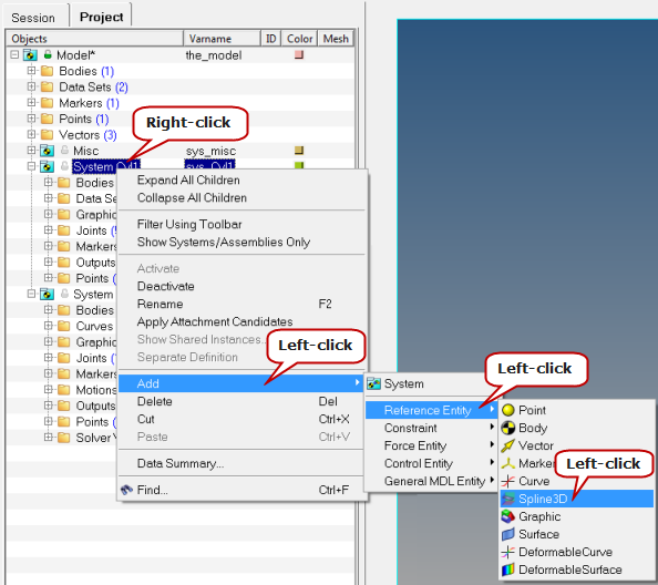
OR
| - | Select System Cyl1 in the Project Browser and then right-click on the Spline3D icon  on the Reference Entity toolbar. on the Reference Entity toolbar. |
The Add Spline3D dialog is displayed.
| 2. | Enter F_ThetaSpline for the Label and spl3d_F_ThetaSpline for the Variable. |
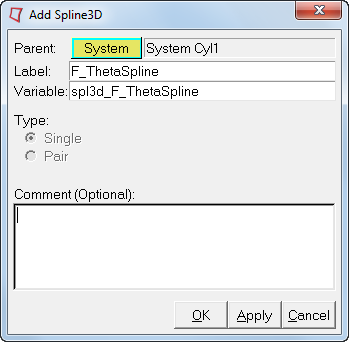
| 3. | Click OK to close the dialog. |
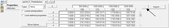
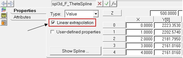
The Spline3D panel is displayed in the panel area with the Properties tab active.
| 4. | Click on the Type drop-down menu and select Value. |
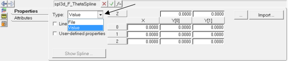
The data for the spline can be defined using either the File or Value methods. For the File type, a reference to an external file in .csv format must be provided. In case of the Value type, the values can be imported from a .CSV file (using Import) or they can be entered in manually. In this tutorial, we will import the values from an external file.
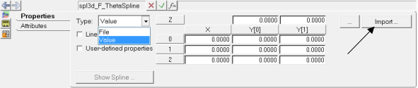
| 5. | Click the Import button to display the Import Values From File dialog. |
| 6. | Browse to the FTheta.csv file in your <working directory> and click OK. |
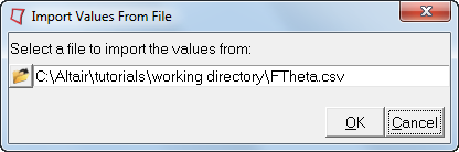
| 7. | In the Warning dialog that appears, click Yes to continue. |
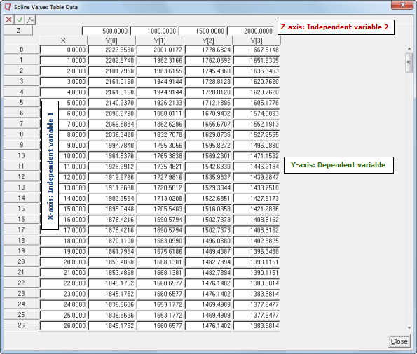
The .csv file that is to be used as the source for Spline3D needs to be in the following format:
| • | The first column must hold the X-axis values (shown in blue below) which is the first independent variable. |
| • | The top row holds the Z-axis values (shown in red below) which is the second independent variable. |
| • | The other columns must have the Y-axis values (shown in green below) with each column belonging to the particular Z-axis values heading that column. |
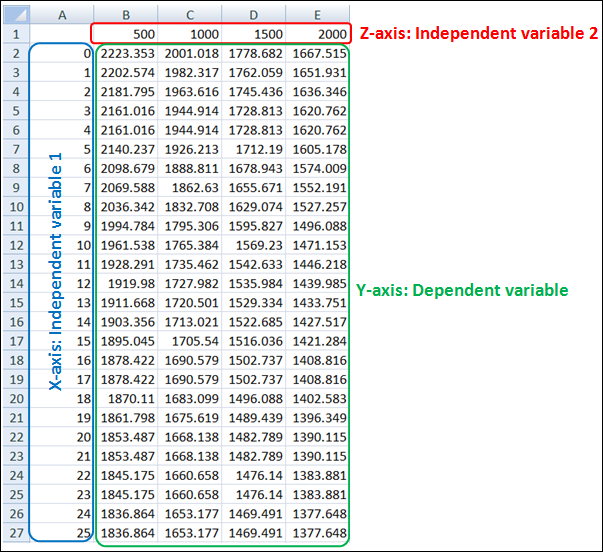
| Note | The same format is applicable when using the File input type. |
| 8. | Once imported, the values are populated in the panel. You may review these by clicking on the Expansion button  in the panel to open the Spline Values Table Data window. in the panel to open the Spline Values Table Data window. |
| 9. | When manually keying in the values, context menus are available which allow you to Insert/Delete/Append row and column data. You can access these menus by right-clicking on any of the row or column headers. If the right-click is made on the last row/column, an Append option will also be available. |
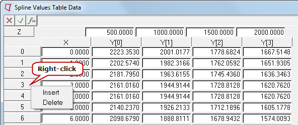
Context Menu (Row)
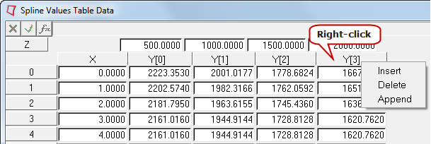
Context Menu (Column)
| 10. | Click Close to close the Spline Values Table Data table. |
| 11. | Activate the Linear Extrapolation check box. This will ensure that the values are extrapolated if the Solver starts looking for values beyond the range of the user provided data. |
| 12. | To visualize the spline graphically, click on the Show Spline button to display the Spline3D viewer dialog. |
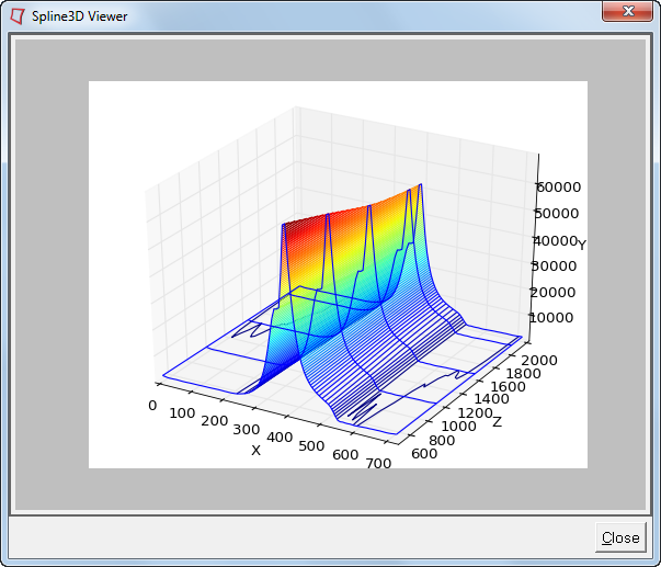
All three axes can be viewed in an isometric view in this window.
| 13. | Click Close to close the viewer. |
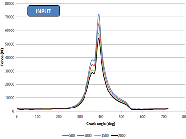
The imported values are Combustion Force on Piston vs Theta (crank angle) diagrams at different speeds (as shown below). The F-Theta profiles vary slightly at different engine or crank speeds. The same plot was visualized in the previous section in the Spline3D viewer by placing the four different plots along the Z-axis.
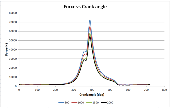
Input Data for Spline3D
Step 3: Adding a force using the Spline3D.
A force will now be added to represent the combustion in the cylinder. This force will be mapped to the Spline3D added in the previous section.
| 1. | Add a Force using one of the following methods: |
| - | From the Project Browser, right-click on System Cyl1 and select Add > Force Entity > Force from the context menu. |
OR
| - | Select System Cyl1 in the Project Browser and then right-click on the Force icon  on the Force Entity toolbar. on the Force Entity toolbar. |
The Add Force or ForcePair dialog is displayed.
| 2. | Enter an appropriate Label and Variable name and click OK. |
The Force panel is displayed in the panel area with the Connectivity tab active.
| 3. | From the Connectivity tab, use the Force drop-down menu to change the type to Action reaction. |
| 4. | Resolve the connections as shown in the image below, either through picking in the graphics area or using the model tree (by double clicking on the input collector). |
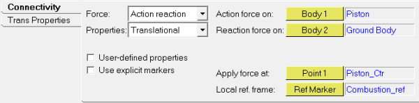
| Note | The Body 2 reference to Ground Body is through an attachment to the System Cyl1 system. |
| 5. | Go to Trans Properties tab and change the Fz type to Spline3D. |
| 6. | Double click on the Spline3D collector,  , to display the Select a Spline3D dialog. , to display the Select a Spline3D dialog. |
| 7. | Select System Cyl1 in the model tree and then navigate to and select the F_ThetaSpline Spline3D (which will then be displayed in the right pane). |
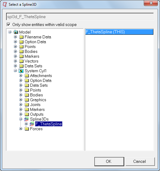
| 8. | Click OK to close the window. |
| 9. | In the Independent variable X field, enter in the following expression: `MOD({arg_Crank_angle_SolVar.VARVAL}, 720)`. |
| 10. | In the Independent variable Z field, enter in the following expression: `{arg_Crank_RPM_SolVar.VARVAL}`. |
| 11. | Click the Check Model button  on the Model Check toolbar to check the model for errors. on the Model Check toolbar to check the model for errors. |
The completed panel is shown below:
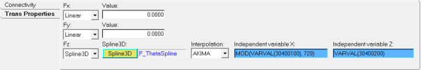
| Note | The solver function MOD() used in Independent variable X refers to the solver variable Crank_angle (deg) in System Flywheel (via attachment arg_Crank_angle_SolVar to System Cyl1). This function calculates the remainder of the division of first argument value (value of the solver variable) by the second argument value (720); thereby resetting the value of Independent variable X every 720 degrees. |
| 12. | Save the model with a different name (File > Save As > Model). |
Step 4: Solving the model and post-processing.
The model is now complete and can be solved in MotionSolve.
| 1. | To solve the model, invoke the Run panel using the Run Solver button  on the General Actions toolbar. on the General Actions toolbar. |
| 2. | Since the crank RPM input data is for 40 seconds, enter 40 in the End time field and change the Print interval to 0.001. |
| 3. | Assign a name and location for the MotionSolve XML file using the browser icon  . . |
| 4. | The Run panel with the inputs from the previous steps is shown below: |
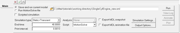
| 5. | Click the Run button in the panel to invoke MotionSolve and solve the model. |
| 6. | Close the solver window after the job is completed. |
| 7. | Click the Animate button in the panel (now active) to load the animation results in a  HyperView window. HyperView window. |
| 8. | From the Animation toolbar, use the Start/Pause Animation button  to animate the model. to animate the model. |
| 9. | Visualize forces on the Piston using the  Vector panel (select the Piston graphics for the Assemblies collector). Vector panel (select the Piston graphics for the Assemblies collector). |
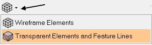
You may also set all graphics to be transparent for easy visualization using the WireFrame/Transparent Elements and Feature Lines option located on the Visualization toolbar.
| 10. | From the Page Controls toolbar, click the Add Page icon  to add a new page. to add a new page. |
| 11. | Use the Select application drop-down menu to change the client on the new page to  HyperGraph 2D. HyperGraph 2D. |
| 12. | From the Page Controls toolbar, click the arrow next to the Page Window Layout button  and select the three window layout and select the three window layout  . . |
| 13. | From the Build Plots panel, use the Data file browser  to load the .plt file from the MotionSolve run. to load the .plt file from the MotionSolve run. |
| 14. | In the first window (top left), plot the Crank_angle (deg) by selecting the following: |
| - | Y Request = REQ/70000003 Crank_angle (deg) |
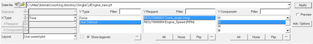
Selections for plotting Crank_angle (deg)
| 15. | Next, click in the graphics area of the second window (top right) to make it the active window and plot the CombustionForce in the Z direction: |
| - | Y Request = REQ/70000002 CombustionForce (ForceOnPiston) |
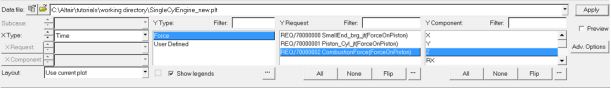
Selections for plotting CombustionForce
| 16. | Finally, we will plot the Force vs Theta plots at different speeds as applied on the piston (this will demonstrate the usage of Spline3D input used in Step 2 of this tutorial). Click in the graphics area of the third window (bottom) to make it the active window. |
| 17. | Click on the Define Curves  icon on the Curves toolbar. icon on the Curves toolbar. |
| 18. | Click the Add button to add a curve. |
| 19. | Click in the Curve field and rename the curve as 500 RPM. |
| 20. | Change the Source to Math. |
| 21. | Enter the expressions shown below to extract the data from the curve in the first and the second window respectively between 6 and 7 seconds. |
| - | x = p2w1c1.y[subrange(p2w1c1.x,6,7)] |
| - | y = p2w2c1.y[subrange(p2w2c1.x,6,7)] |
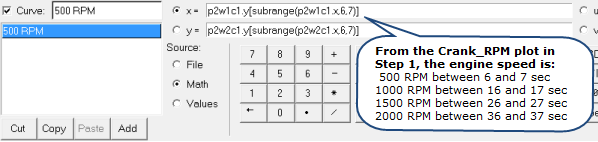
Panel entries for plotting Force vs Theta
| Note | p2w1c1 refers to the Curve 1 plotted on Page 2, Window 1. If for any reason the page, window, or curve numbering is different, suitable modifications should be made to the expression. |
The subrange function returns the indices of the vector within a specified range. For more information on the subrange function, please refer to the Templex and Math Reference Guide.
| 23. | Similarly, add three more plots for 1000, 1500, and 2000 RPM. Use time values of: 16, 17; 26, 27; and 36, 37 respectively (in place of 6, 7 shown in the expression above). |
| 24. | Assign different colors to these curves using the Curve Attributes panel  , or by selecting the curves in the Plot Browser and changing the color in the Properties table. , or by selecting the curves in the Plot Browser and changing the color in the Properties table. |
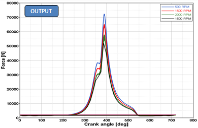
| 25. | After completing the plots, compare them with the input data for the Spline3D plot in Step 2. A comparison is shown below: |
Validating the Spline3D used by the Solver