The objective of this tutorial is to replace several entities in a MotionView model with Python user subroutines. You will run a model initially, and then edit the file to incorporate Python scripts in place of MotionView entities and compare the results from each simulation.
In this tutorial, you will learn how:
| • | User subroutines are incorporated into MotionView |
| • | User subroutines are useful in customizing models |
| • | To create Python scripts that can be used to define these subroutines (and how they are called by MotionView). |
You must be familiar with the MotionView user interface and entities panel, as well as have some experience defining and modifying entities. Some experience with the Python programming language is necessary to fully understand the topics covered.
Exercise One - Introduction to User Subroutines
User subroutines are a useful tool to customize simulations and analyses. These subroutines, or usersubs can be created using variety of programming languages like C, Ruby, TCL, and Python. Subroutines created in programming languages like C, C++ and FORTRAN etc. are compiled to create *.dll files using the MS UserSub Build Tool (located in the MotionView Tools menu). These dlls are then used by the solver. In older versions of MotionView only compiled usersubs (*.dll) were supported. Starting with MotionView version 11.0, usersubs are enabled to use Python and Matlab scripts. In this tutorial, we will be using Python to create usersubs. User subroutines can make use of external Python scripts in order to define complex simulations, which cannot be created through the MotionView GUI. With a basic knowledge of the Python programming language, a user can easily generate intricate experiments to simulate any complex mechanism.
This tutorial will show you how to replace five MotionView entities with their corresponding usersubs.
Copy the model file required for this exercise, engine_baseline.mdl, along with all of the H3D files located in the mbd_modeling\motionsolve\python_usersub folder to your <working directory>.
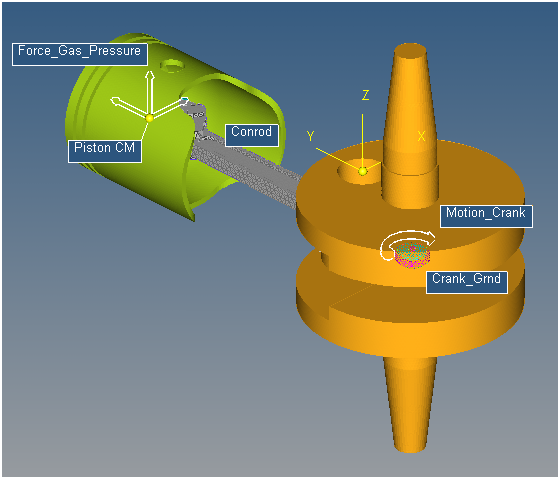
The single cylinder engine model
The model we are using is a single cylinder engine, and uses a curve, an output, a force, and a motion entity. The system also uses default damping.
| • | The curve is read from a CSV file, and gives a force value based on the angular displacement of the connecting rod. |
| • | The output returns the displacement magnitude of the piston. |
| • | The force entity uses the angle of the connecting rod and the curve to apply a variable pressure force to the piston. |
| • | The motion entity applies an angular motion to the Crank_Grnd revolute joint. |
| • | The default damping of the system is 1, however it can be changed in the Bodies panel. |
The following is a list of the entities and usersubs we will be using in this tutorial, along with a brief description of their usage:
|
Entity
|
Usrsub
|
Description
|

|
Curve
|
SPLINE_READ
|
Reads the curve data file.
|

|
Request
|
REQSUB
|
Outputs the requested values
|

|
Force
|
GFOSUB
|
Applies a force on the system.
|

|
Motion
|
MOTSUB
|
Applies a motion to the system.
|

|
Damping
|
DMPSUB
|
Defines the damping of a flexbody.
|
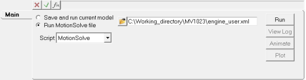
Step 1: Running the model.
| 1. | Click the Run panel icon,  , to access the Run panel. , to access the Run panel. |
| 2. | Click on the folder icon located next to the Save and run current model option, and browse to your <working directory>. Specify the name as engine_baseline.xml for the MotionSolve input XML file. |
| 3. | Check your model for errors, and then click the Run button to run your model. |
This will give you result files to compare with your usrsub results.
Exercise Two - Adding User Subroutines
Notes on using XML syntax in Python
Python can use many MotionSolve functions and inputs when certain syntax rules are followed. When using a MotionSolve function such as AKISPL or SYSFNC, the string “py_” must be added to the beginning. For example, “py_sysfnc(…” would be the correct usage of SYSFNC in Python. When defining a usersub function in Python, the name of the function and the inputs must match those outlined in the MotionSolve online help pages exactly. When accessing model data in python through a function such as SYSFNC, use the exact property name in quotations as the “id” input. Model properties that are passed into Python in the function definition can be accessed throughout the script, and do not need additional defining to use. An example of these syntax rules being used is shown below:
def REQSUB(id, time, par, npar, iflag):
[A, errflg] = py_sysfnc(“DX”,[par[0],par[1]])
return A
Step 1: Using SPLINE_READ to Replace the Curve Entity.
The first user-subroutine we will implement uses the SPLINE_READ function to return the curve from the included pressure_curve.csv file. SPLINE_READ is the usersub that corresponds to the curve entity in MotionView. It uses data points in an external file to create a curve, which can then be used by other entities.
Writing the Python script:
| 1. | Open a new Python file, and define a function with the name SPLINE_READ using “def SPLINE_READ():", giving the appropriate inputs and outputs. The inputs and outputs used are: id, file_name, and block_name. |
| 2. | Import the Python CSV package by including import csv after the function definition. |
| 3. | Open pressure_curve.csv in the function, and read the file to your Python script as a variable. This can be done with “variable = open(‘pressure_curve.csv’, ’r’)”. |
| 4. | Change the format of this variable from csv by defining a new variable, and using csv.reader() to read your variable file. |
| 5. | Define an empty list, “L”, to store the pressure_curve data values. Iterate through the list using “for item in curv:”. Append each item as a separate list value with “L.append(item)”. |
| 6. | Remove the headers from the csv file by redefining the list from the second value till the end of the list. This can be done with “L = L[1:]”. |
| 7. | Define a counter variable to be used later. Define two lists that are half the length of “L”, and set them equal to zero. To do this, use “x = 16*[0.0]” twice; once with the x value and once with the y value. |
| 8. | Create a while loop dependent on your counter variable being less than the length of your list, minus one. |
| 9. | In each iteration of the loop, define your x and y data values for the index “i” as a floating value of each half of your “L” data sets. This should look like “x[i] = float(L[i][0])” and “y[i] = float(L[i][1])”. Increase your counter variable by 1. |
| 10. | Define a z variable with a floating value of 0.0, and close the csv file. Defining a z variable is necessary, as the next function we will use requires an x, y, and z variable. |
| 11. | Use the put_spline MotionSolve function, and return the “id”, as well as the lists containing the first and second column of values and the z variable. This should be done with “errflg = py_put_spline(id,x,y,z)” followed by “return errflg”. |
| 12. | Save this file to your working directory as nonlin_spline.py. |
Your nonlin_spline.py Python script should resemble the following:
def SPLINE_READ(id, file_name, block_name):
import csv
ifile= open('pressure_curve.csv','r') ## opens data file as readable variable
curv = csv.reader(ifile) ## reads csv data, stores as useable var.
L = [] ## creates empty list
for item in curv:
L.append(item) ## separates file values into list
L = L[1:] ## removes block names from list
i=0 ## creates counter
x = 16*[0.0]
y = 16*[0.0] ## splits list into x and y lists
while i < (len(L)-1):
x[i] = float(L[i][0]) ## changes values from str to float
y[i] = float(L[i][1])
i+=1 ## counter increment
z = 0.0 ## defines z value
ifile.close() ## closes data file
errflg = py_put_spline(id,x,y,z) ## var to create MotionSolve spline
return errflg ## returns var
Implementing the Python script:
| 1. | In MotionView, go to the Curve panel , and locate the Force_Pressure curve in the project directory tree to the left of the MotionView workspace. |
| 2. | From the Properties tab, check the box marked User-defined. |
| 3. | From the Attributes tab, make sure Linear extrapolation is checked. |
| 4. | Click on the User-Defined tab, and use the File name file browser to select the pressure_curve.csv file. |
| 5. | Check the box marked Use local file and function name. Use the Local File file browser (the folder button to the right) to locate and select the nonlin_spline.py file. |
| 6. | Change the Function Type in the drop-down menu from DLL to Python, and ensure the function name is SPLINE_READ. You do not need to enter anything for the Block name, as it is not needed in this tutorial. |
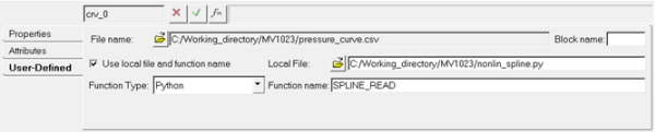
The curve panel using the SPLINE_READ usersub
Step 2: Using REQSUB to Request an Output.
The second user-subroutine will use Python to specify which values to return. In this tutorial, the returned values will be the magnitude of displacement for the piston.
Writing the Python script:
| 1. | Create another Python file, and define a function named REQSUB with the appropriate inputs and outputs. The syntax for this is “def REQSUB(id, time, par, npar, iflag)”. |
| 2. | Use the sysfnc utility to implement the “DM” (or displacement magnitude) function on the first and second input parameters, and define a variable and an error flag by writing “[D, errflg] = py_sysfnc(“DM”,[par[0],par[1]])”. |
| 3. | Return a list of eight values, where the second value is your variable, and the rest are equal to 0. This will be your result variable, and should look like “result = [0,D,0,0,0,0,0,0]”. |
| 4. | Save this file to your working directory as req_nonlin.py. |
Your req_nonlin.py Python script should resemble the following:
def REQSUB(id, time, par, npar, iflag):
[D, errflg] = py_sysfnc("DM",[par[0],par[1]]) ## sets "D" as piston displacement mag
result = [0,D,0,0,0,0,0,0] ## lists results for output return
return result ## sends list with results to motionsolve as output
Implementing the Python script:
| 1. | In MotionView, go to the Outputs panel , and locate the Output_Conrod_Length output in the project directory tree to the left of the MotionView workspace. |
The Outputs panel is displayed.
| 2. | From the Properties tab, select User Defined from the first drop-down menu. |
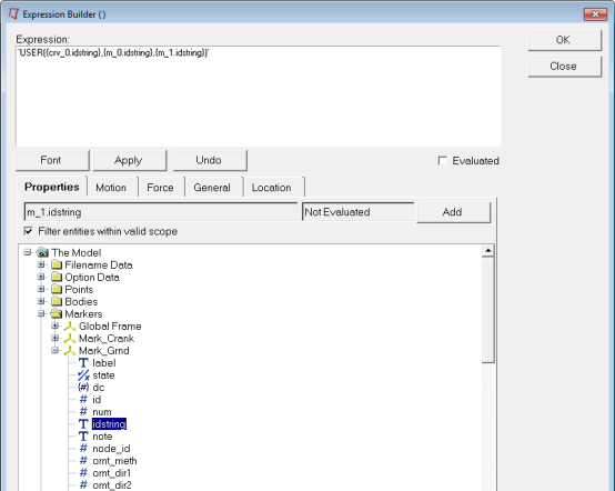
| 3. | Click in the text field labeled Output, and then click on the  button to open the Expression Builder. button to open the Expression Builder. |
| 4. | In the text field of the Expression Builder, click inside the parentheses and add “{},{}”. |
| 5. | From the Expression Builder, locate and select the j_0.i.idstring (located in the Joints folder in the directory) and insert this id string into the expression by positioning the cursor inside a set of braces and clicking the Add button. In addition, add the j_1.i.idstring into the expression by repeating this same process. |
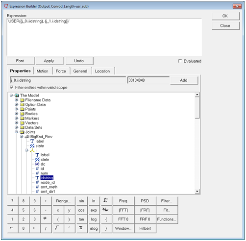
Expression Builder dialog
| 6. | Click OK to close the dialog. |
| 7. | Check the Use local file and function name box, and select Python from the Function Type drop-down menu. |
| 8. | Use the Local File file browser to locate and select the req_nonlin.py script, and make sure that the Function name text field reads REQSUB. |
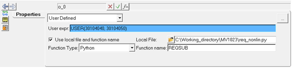
Outputs panel using REQSUB
Step 3: Using GFOSUB to Replace the Force Entity.
The GFOSUB user subroutine replaces a force with a user defined Python script. The GFOSUB used here will take the curve data defined with SPLINE_READ, and change depending on the Conrod angle according to the curve.
Writing the Python script:
| 1. | Open a new Python file, and define the function GFOSUB by typing “def GFOSUB(id, time, par, npar, dflag, iflag):”. |
| 2. | Import "pi" from the Python “math” library using “from math import pi”. |
| 3. | Use the “AZ” function for angle in the z direction with the sysfnc command, to save it as a variable. To do this, type “[A, errflg] = py_sysfnc(“AZ”,[par[1],par[2]])”. |
| 4. | The angle will be measured in radians by default, so change the variable defined in the previous step to degrees. As the model extends from the origin into the negative y direction, you will need to multiply by -1. The method used in this tutorial is “B = ((-1)*A*180)/pi”. |
| 5. | Define another variable using the “akispl” utility, which interpolates the force values from the curve. You will need input arguments of your angle “B”, zero to specify a two dimensional curve, and zero for the curve input and the order. This line is written as “[C, errflg] = py_akispl(B,0,par[0],0)”. |
| 6. | Return a list three elements long, where the second element is the variable defined with the Akima interpolation function. The data from interpolation is stored in the first column, so use “return [0,C[0],0]”. |
| 7. | Save this file to your working directory as gfo_nonlin.py. |
Your gfo_nonlin.py Python script should resemble the following:
def GFOSUB(id, time, par, npar, dflag, iflag):
from math import pi
[A, errflg] = py_sysfnc("AZ",[par[1],par[2]]) ## retreives conrod angle
B = ((-1)*A*180)/pi ## converts radians to degrees
[C, errflg] = py_akispl(B,0,par[0],0) ## interpolates data to fit curve
return [0,C[0],0] ## returns C data as force values
Implementing the Python script:
| 1. | In MotionView, go to the Forces panel , and locate the Force_Gas_Pressure force in the project directory tree to the left of the MotionView workspace. |
| 2. | From the Connectivity tab, check the User-defined properties box. |
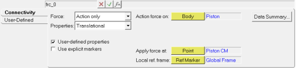
| 3. | From the User-Defined tab, edit the Force value with the Expression Builder to include the curve idstring, the ground marker idstring, and the crank marker idstring. |
| 4. | Click OK to close the dialog. |
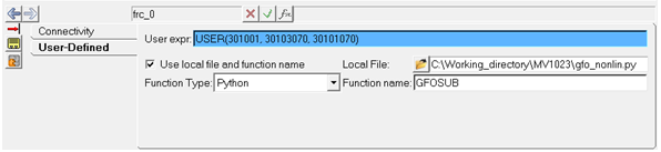
| 5. | Check the Use local file and function name box, and select Python from the Function Type drop-down menu. |
| 6. | For Local File, select gfo_nonlin.py from your working directory. |
| 7. | Make sure the Function name is set to GFOSUB. |
Step 4: Using MOTSUB to Define a Motion.
Writing the Python script:
| 1. | Open a new python file, and define the MOTSUB function, including the required inputs. The correct syntax for this is “def MOTSUB(id, time, par, npar, iord, iflag):”. |
| 2. | The MOTSUB user subroutine requires a function or expression, and its first and second order derivatives. Create conditional statements using the function order variable “iord” to define the function and its first and second derivatives with “if iord==0:”, “elif iord==1:” and “else:”. |
| 3. | The function and its derivatives should be defined with the same variable name. The function used in this tutorial is “A = 10.0461*time”. This makes the first derivative equal to “A = 10.0461”, and the second derivative equal to “A = 0.0”. |
| 4. | Return the function variable with “return A”. |
| 5. | Save this file to your working directory as mot_nonlin.py. |
Your mot_nonlin.py Python script should resemble the following:
def MOTSUB(id, time, par, npar, iord, iflag):
if iord==0: ## function
A = 10.0461*time
elif iord==1: ## first derivative
A = 10.0461
else: ## second derivative
A = 0.0
return A ## returns function based on iord input
Implementing the Python script:
| 1. | In the directory tree on the left side of the HyperWorks desktop, locate the Motion_Crank motion and click on it. |
The Motions panel is displayed.
| 2. | In the Motions panel, check the User-defined properties box. |
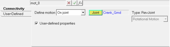
| 3. | Click on the User-Defined tab. |
Because we defined the function in the Python script, we do not need to modify USER() text field.
| 4. | Check the box labeled Use local file and function name, select Python from the Function Type drop-down menu. |
| 5. | Use the Local File file browser to locate and select the mot_nonlin.py file. |
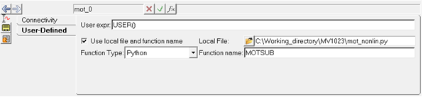
Motions panel using MOTSUB
Step 5: Using DMPSUB to Add Custom Flexbody Damping.
Writing the Python script:
| 1. | Open a new Python file and define the DMPSUB function with “def DMPSUB():”, giving it the following inputs: “id, time, par, npar, freq, nmode, h”. |
| 2. | Define a list the length of “nmode” using “cratios = nmode*[0.0]”. |
nmode is the number of modes in the flexbody.
| 3. | Create an “if” statement to iterate along the list of modes in the flexbody. The “xrange()” function can be used here, resulting in “for I in xrange(nmode):”. |
| 4. | In each iteration of the loop, set each index in your variable equal to 1 by adding “cratios[i] = 1.0”. |
| 5. | At the end of your script, return the list variable with “return cratios”. |
| 6. | Save your script as dmp_nonlin.py. |
Your dmp_nonlin.py Python script should resemble the following:
def DMPSUB(id, time, par, npar, freq, nmode, h):
cratios = nmode*[0.0] ## makes preallocated list for markers
for i in xrange(nmode):
cratios[i] = 1.0 ## sets marker damping to 1
return cratios ## returns damping values
Implementing the Python script:
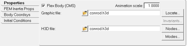
| 1. | In the directory tree on the left side of the HyperWorks desktop, locate the Conrod body and click on it (this is a flexbody in the model). |
| 2. | From the Properties tab, click on the Modes… button (located in the lower right corner of the panel) to display the Modes dialog. |
| 3. | Use the drop-down menu to select the User Function Damping option. |
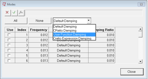
Because we defined the damping in our dmp_nonlin.py script, we do not need to change the USER() expression.
| 4. | Go to the Run panel . |
| 5. | Change the End time to 5.0, and the Print interval to 0.01. |
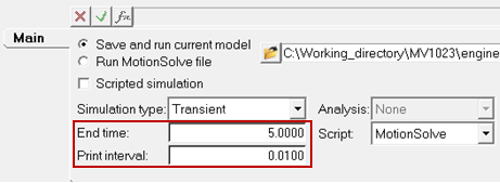
| 6. | Now, export the MotionSolve file using File > Export > Solver Deck. |
| Note | Currently there is no GUI option available to specify the DAMPSUB file defining flexbody damping, therefore the dmp_nonlin.py must be manually added to the MotionSolve file (*.xml) by adding following statements to the flexbody definition: |
is_user_damp = "TRUE"
usrsub_param_string = "USER()"
interpreter = "Python"
script_name = "dmp_nonlin.py"
usrsub_fnc_name = "DMPSUB"
Your flexbody definition should look like below:
<Body_Flexible
id = "30104"
lprf_id = "30104002"
mass = "7.424574879203591E-02"
inertia_xx = "1.471824534365642E+02"
inertia_yy = "4.505004745855096E+00"
inertia_zz = "1.501914135052064E+02"
inertia_xy = "-5.546373592613223E-03"
inertia_yz = "-1.984540442733755E-03"
inertia_xz = "1.557626595859531E-03"
cm_x = "1.191728011928773E-03"
cm_y = "-2.225471002399553E+01"
cm_z = "5.469513396916666E-05"
h3d_file = "conrod.h3d"
is_user_damp = "TRUE"
usrsub_param_string = "USER()"
interpreter = "Python"
script_name = "dmp_nonlin.py"
usrsub_fnc_name = "DMPSUB"
flexdata_id = "30104"
animation_scale = "1."
/>
Exercise Three - Running Your Simulation with Usersubs
Now that all the user subroutines have been implemented, run your model, and compare your results to those from your initial test.
Step 1: Using the Run Solver Panel to Run Your Model.
| 1. | Go to the Run panel , click on/activate the Run MotionSolve file radio button. |
| 2. | Now browse to the *.xml file saved in previous step. |
Exercise Four - Comparing Your Results
Now that we have results for both the initial model and the model using user subroutines, we will compare the data to ensure accuracy. We will do this using HyperGraph and Hyperview to compare the outputs and deformations of the system.
Step 1: Using HyperGraph to Plot the Displacement Magnitudes.
Using the outputs from both simulations, we will compare the displacement magnitude of the piston. A correct result from the usersub run will match the results from the initial run.
| 1. | Begin by opening a new window by clicking the Add Page button  . . |
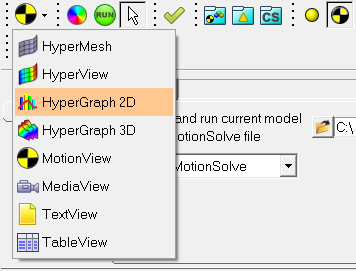
| 2. | Switch the application from MotionView to HyperGraph 2D by selecting it from the Client Selector drop-down menu  (located on the left-most end of the Client Selector toolbar). (located on the left-most end of the Client Selector toolbar). |
| 3. | In HyperGraph, click the Build Plots panel button  on the Curves toolbar. on the Curves toolbar. |
| 4. | In the Build Plots panel, locate your baseline results from your working directory using the Data file file browser. Select the file baseline.abf, and click Open. |
| 5. | The x and y axes options are be shown below. The default x variable is Time. For the y variable: select Marker Displacement for Y Type, leave the default for Y Request, and select DM for Y Component. |
| 6. | Click the Apply button (located on the far right side of the panel). |
| 7. | For your usersub results, repeat steps 4 through 6, using REQSUB and RESULT(2) for Y Type and Y Component respectively. |
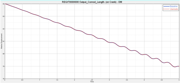
Comparison of output results from both model simulations
Step 2: Using HyperView to Compare Flexbody Stresses.
Using HyperView, you can view the stresses and deformations on the flexbody. The results between the two simulations should be the same.
| 1. | Add a new window by clicking the Add Page button . |
| 2. | Switch the application from HyperGraph 2D to HyperView using the Client Selector drop-down menu. |
| 3. | Click the Load Results button  on the Standard toolbar. on the Standard toolbar. |
| 4. | Locate your baseline.h3d results file in your working directory, and click Open. |
| 6. | Open the Entity Attributes panel  , and click the Off button next to the Display option. Make sure that the Auto apply mode check box is checked. , and click the Off button next to the Display option. Make sure that the Auto apply mode check box is checked. |
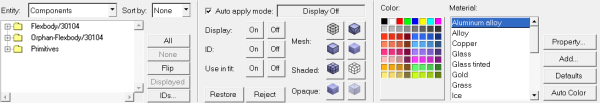
| 7. | In the model window, click on the piston head, and both crank components. |
Only the flexbody component should be displayed.
| 8. | Click the Contour panel button  located on the Results toolbar. located on the Results toolbar. |
The Contour panel is displayed.
| 9. | Set Result type to Deformation->Displacement (v), and click on the flexbody in the model window. |
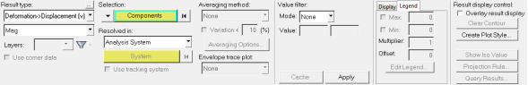
| 10. | Click the Apply button (located in the lower middle portion of the panel). |
| 11. | Next, click on the Tracking Systems panel button  located on the Results toolbar. located on the Results toolbar. |
| 12. | From the Track drop-down menu, select Component, then click on the flexbody in your model window. |
| 13. | Separate your model window into two halves using the Page Window Layout drop-down menu  (located on the Page Controls toolbar). (located on the Page Controls toolbar). |
| 14. | In the blank model window, repeat steps 3 through 12 for your usersub h3d file. |
| 15. | Click on the Start/Pause button  on the Animation toolbar to animate your models. on the Animation toolbar to animate your models. |
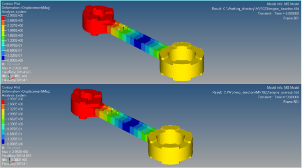
Comparison of flexbody deformation in HyperView


