HyperStudy

HS-1035: Optimization Study Using an Excel Spreadsheet

HS-1035: Optimization Study Using an Excel Spreadsheet

Previous topic Next topic Expand/collapse all hidden text  

HS-1035: Optimization Study Using an Excel Spreadsheet

Previous topic Next topic JavaScript is required for expanding text JavaScript is required for the print function  

In this tutorial, you will learn how to:

Couple HyperStudy with a spreadsheet.
Identify input variables and output responses.
Set up an Optimization study.
Analyze Optimization results.


Problem formulation:

Find the cross-sectional dimension's width and height in mm.
Minimize the beam volume such that the tip deflection < 0.53 mm.


The Excel spreadsheet used in this tutorial can be found in <hst.zip>/HS-1035/. Copy the file from this directory to your working directory.

hmtoggle_plus1greyStep 1: Review the Excel Spreadsheet
1.In Excel, open the hst_tut_1035(1070)_spreadsheet.xls file.
2.Review the information, and locate the columns that contain the input variables and output responses.
Note:When you create an Excel spreadsheet model, it is important that the spreadsheet is formatted correctly. A variable's value and label can be formatted in two consecutive rows or two consecutive columns. Variable labels should only contain English characters, or a combination of English characters and numbers. If a label is not created for a variable, HyperStudy will assign one by default.


hmtoggle_plus1greyStep 2: Perform the Study Setup
1.Start HyperStudy.
2.To start a new study, click File > New from the menu bar, or click files_new_hst2 on the toolbar.
3.In the HyperStudy – Add dialog, enter a study name, select a location for the study, and click OK.
4.Go to the Define Models step.
5.Add a Spreadsheet model by dragging-and-dropping the hst_tut_1035(1070)_spreadsheet.xls file from the Directory into the work area.

hs_1035_drag_drop_model

The Resource, Solver input file, and Solver input arguments fields become populated. The Solver input file field displays hst_input.hstp, this is the name of the solver input file HyperStudy writes during an evaluation.

hs_1035_define_model

6.Click Import Variables. The hst_tut_1035(1070)_spreadsheet.xls spreadsheet opens.
7.Add input variables.
a.In the Excel - HyperStudy dialog, click Yes to begin selecting input variables.

hs_1035_excel_dialog

b.In the spreadsheet, select the cells that contain the input variable's labels and values.

new_hs_1070_1

c.In the Excel - HyperStudy Input selector dialog, click OK.
d.Click Cancel to stop selecting input variables.
8.Add output responses.
a.In the Excel - HyperStudy dialog, click Yes to begin selecting output responses.
b.In the spreadsheet, select the cells that contain the output response's labels and values.

hs_1035_output

c.In the Excel - HyperStudy Output selector dialog, click OK.
d.Click Cancel to stop selecting output responses. Two input variables and two output responses are imported from the hst_tut_1070_spreadsheet.xls spreadsheet.
9.Go to the Define Input Variables step.
10.Review the input variable's lower and upper bound ranges.
11.Go to the Specifications step.


hmtoggle_plus1greyStep 3: Perform the Nominal Run
1.In the work area, set the Mode to Nominal Run.
2.Click Apply.
3.Go to the Evaluate step.
4.Click Evaluate Tasks. An approach/nom_1/ directory is created inside the study directory. The approaches/nom_1/run__00001/m_1 directory contains the sse_output.csv file, which is the result of the nominal run.
5.Go to the Define Output Responses step.


hmtoggle_plus1greyStep 4: Create and Define Output Responses

Review the output responses imported into the study. The output responses were extracted from the hst_output.hstp file, which HyperStudy created for each run.

hs_1035_expression


hmtoggle_plus1greyStep 5: Run an Optimization Study
1.In the Explorer, right-click and select Add Approach from the context menu.
2.In the HyperStudy - Add dialog, select Optimization and click OK.
3.Go to the Select Input Variables step.
4.Apply a set range of +17% to both input variable's lower and upper bounds.
a.In the Lower Bound column of both input variables, click hs_popupdialogicon.
b.Under Set Range, in the Percent field, enter +17.
c.Click the +/- button.
d.Click Apply.

hs_1035_define_optimization

5.Go to the Select Output Responses step.
6.Add an objective.
a.Click the Objectives tab.
b.Click Add Objective.
c.In the HyperStudy - Add dialog, add one objective.
d.Define the objective.
Set Type to Minimize.
Set Apply On to Beam Volume (m^3) (r_2).

1035_r2a

7.Add a constraint.
a.Click the Constraints tab.
b.Click Add Constraint.
c.In the HyperStudy - Add dialog, add one constraint.
d.Define the constraint.
Set Apply On to Deflection at the tip (mm) (r_1).
Set Bound Type to <= (less than or equal to).
For Bound Value, enter 0.53.

bound_value

8.Click Apply.
9.Go to the Specifications step.
10.In the work area, set the Mode to Adaptive Response Surface Method (ARSM).
Note:Only the methods that are valid for the problem formulation are enabled.
11.Click Apply.
12.Go to the Evaluate step.
13.Click Evaluate Tasks.
14.Optional.
To stop the optimization, click hs_stop.
To monitor the progress of the Optimization, click the Task tab.


hmtoggle_plus1greyStep 6: View the Evaluation Data and Plot of an Optimization Approach

Use the Evaluation Data and Evaluation Plot tabs to review the values of input variables, output responses, objective functions, and constraints for all runs evaluated during the optimization.

hs_1035_7


hmtoggle_plus1greyStep 7: View the Iteration History and Plot of an Optimization Approach

Use the Iteration History and Iteration Plot tabs to review the values of input variables, output responses, objective function, and constraints for each iteration during the optimization.
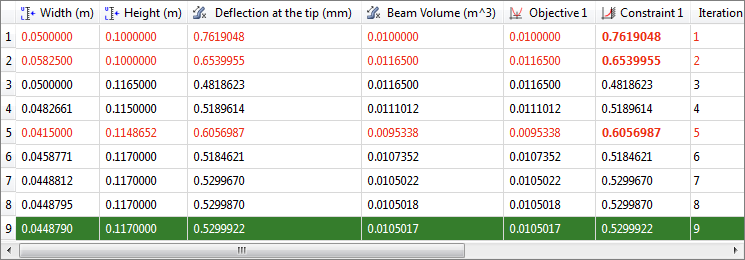
1.Click the Iteration History tab to view the iteration history results in a table.

As this study was run with ARSM, you will see the same designs in both the Evaluation Data and Iteration History. From the iteration table, you can see that iterations 1, 2, and 5 are displayed in a red font, which indicates that these iterations have a constraint violation. The constraint that is violated, Constraint 1, is displayed in a red, bold font. Iterations 3, 4, and 6-8 are feasible, but not optimal designs. The ninth iteration, highlighted in green, indicates that this design is the optimal design.
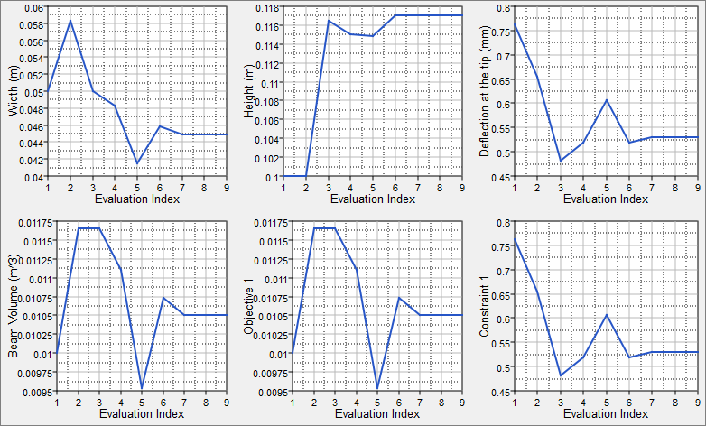
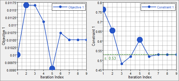
hs_1035_6

2.Click the Iteration Plot tab to view the iteration history results in a plot.

Use the Channel selector to select Objective 1 and Constraint 1.
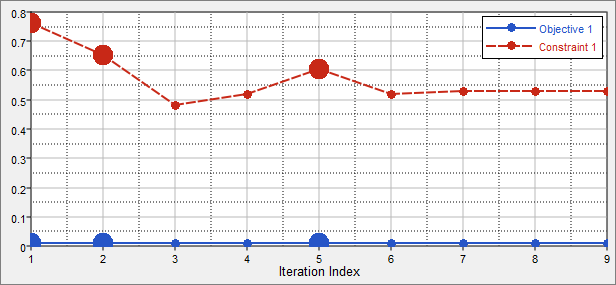
1035_9

3.To view a single plot that contains the iteration history of Objective 1 and Constraint 1, click single_plot1. In the Objective plot, infeasible designs are identified with bigger markers. In the Constraint plot, you can see these designs have higher displacement value than the constraint bound of 0.53 and only the last three designs meet the constraint bound.

1035_8


See Also:

HyperStudy Tutorials