HS-1525: Simple Optimization Study Using HyperMath Functions in HyperStudy

HyperStudy can be connected to HyperMath by either using HyperMath as a solver (as in this tutorial) or by registering HyperMath functions to be used in HyperStudy’s evaluation.

In this tutorial, you will learn how to use HyperMath within an optimization study. The example consists of optimizing a 2-dimensional Rosenbrock function. HyperMath is seen as a solver for HyperStudy, and the HyperMath function file (.hml) is the model. This example defines two input variables, labeled x and y, respectively. The objective of the optimization is to minimize f(x,y)= 100*(y-x^2)^2 + (1-x)^2. The range for x and y is set to [-2 ; 2], and the start point is [1.2 ; 1.1].

1.	Start HyperMath.

2.	From the menu bar, click File > New.

3.	In the Create New File dialog, select HyperMath File.

4.	Click OK. A new .hml file opens.

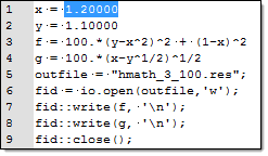
5.	In the editor, enter the following HyperMath commands:

HyperMath commands	Explanation
x = 1.20000	Set the value of variable x.
y = 1.10000	Set the value of variable y.
f = 100.*(y-x^2)^2 + (1-x)^2	Compute Rosenbrock function.
g = 100.*(x-y^1/2)^1/2	Compute any other function (not used in this tutorial).
outfile = "hmath_3_100.res";	Define a result file.
fid = io.open(outfile,'w');	Open the result file in Write mode.
fid::write(f, '\n');	Write to file the current value of function f.
fid::write(g, '\n');	Write to file the current value of function g.
fid::close();	Close the result file.

6.	From the menu bar, click File > Save As.

7.	In the Save As dialog, save the file as HMath_3_100.hml.

8.	Quit HyperMath by clicking File > Exit from the menu bar.

1.	Start HyperStudy.

2.	From the menu bar, click Tools > Editor. The HyperStudy - Editor opens.

3.	In the File field, open the HMath_3_100.hml file.

4.	Highlight the x= value, 1.20000.

hmath2

5.	Right-click on the highlighted fields and select Create Parameter from the context menu.

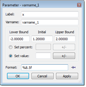
6.	In the Parameter - varname_1 dialog, Label field, enter X.

7.	Set the Lower bound to -2.00000, the Initial value to 1.20000, and the Upper bound to 2.00000.

8.	Set the Format to %8.5f.

Click OK.

hmath_dvprops1

10.	Highlight the y= value, 1.10000.

11.	Right-click on the highlighted fields and select Create Parameter from the context menu.

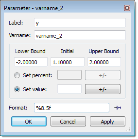
12.	In the Parameter - varname_2 dialog, Label field, enter y.

13.	Set the Lower bound to -2.00000, the Initial value to 1.10000, and the Upper bound to 2.00000.

14.	Set the Format to %8.5f.

15.

Click OK.

hmath_dvprops2

16.	Click Save.

17.	In the Save Template dialog, save the file as HMath_3_100.tpl.

18.	Close the HyperStudy - Editor dialog.

1.	To start a new study, click File > New from the menu bar, or click on the toolbar.

2.	In the HyperStudy – Add dialog, enter a study name, select a location for the study, and click OK.

3.	Go to the Define models step.

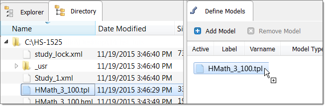
4.	Add a Parameterized File model.

a.	From the Directory, drag-and-drop the HMath_3_100.tpl file into the work area.

hs_1525_drag_drop_model

b.	In the Solver input file column, enter HMath_3_100.hml. This is the name of the solver input file HyperStudy writes during any evaluation.

c.	In the Solver execution script column, select HyperMath (hmath).

d.	In the Solver input arguments column, enter -f infront $file.

Note:

For solver scripts running on Linux, enter "-f $file -nobg" in the Solver input arguments column to ensure that the HyperMath batch mode runs in the foreground instead of the background.

hs_1525_define_models

5.	Click Import Variables. Two input variables are imported from the HMath_3_100.tpl file.

6.	Go to the Define Input Variables step.

7.	Review the input variable's lower and upper bound ranges. The attributes that you defined when you created the template file are now exposed.

8.	Go to the Specifications step.

1.	In the work area, set the Mode to Nominal Run.

2.	Click Apply.

3.	Go to the Evaluate step.

4.	Click Evaluate Tasks.

5.	Go to the Define Output Responses step.

In this step you will create two output responses.

1.	Create output response 1.

a.	From the Directory, drag-and-drop the hmath_3_100.res file, located in the approaches/nom_1/run__00001/m_1 directory, into the work area.

b.	In the File Assistant dialog, set the Reading technology to Altair® HyperWorks® and click Next.

c.	Select Single item in a time series, then click Next.

d.	Define the following options, and then click Next.

•	Set Type to unknown.

•	Set Request to Block 1.

•	Set Component to Column 1.

hs_1525_vector1

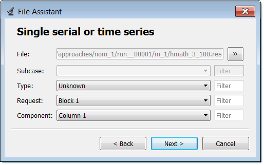
e.	Optional. Enter labels for the vector source and output response.

f.	Set Expression to First Element. The expression changes to m_1_v_1[0].

hs_1525_evalexp

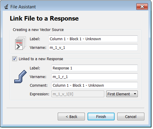
g.	Click Finish. Output response 1 is added to the work area.

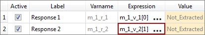
2.	Create output response 2 by repeating step 1.

3.	In the Expression field for Response 2, select the second value by changing the [0] to [1] after v_2.

hs_1010_change_expression

4.	Click Evaluate Expressions. This completes the study setup.

1.	In the Explorer, right-click and select Add Approach from the context menu.

2.	In the HyperStudy - Add dialog, select Optimization and click OK.

3.	Go to the Select Input Variables step.

4.	Review the input variable's lower and upper bound ranges.

5.	Go to the Select Output Responses step.

6.	Click Add Objective.

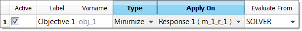
7.	In the HyperStudy - Add dialog, add one objective.

8.	Define the objective.

a.	Set Type to Minimize.

b.	Set Apply On to Response 1 (r_1).

hs_1525_objective

9.	Click Apply.

10.	Go to the Specifications step.

11.	In the work area, set the Mode to Adaptive Response Surface Method (ARSM).

Note:

Only the methods that are valid for the problem formulation are enabled.

12.	Click Apply.

13.	Go to the Evaluate step.

14.	Click Evaluate Tasks.

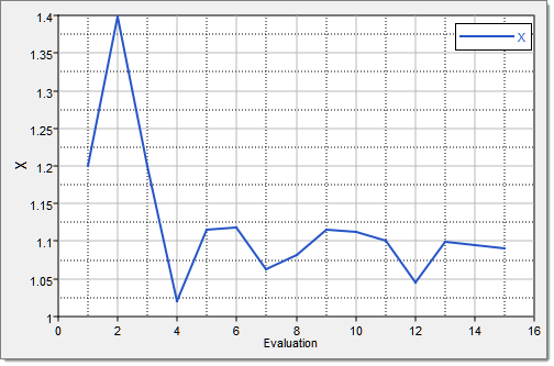
15.	Click the Evaluation Plot tab to monitor the progress of the optimization.

evolution_plot0040

HS-1525: Simple Optimization Study Using HyperMath Functions in HyperStudy

HS-1525: Simple Optimization Study Using HyperMath Functions in HyperStudy

HS-1525: Simple Optimization Study Using HyperMath Functions in HyperStudy

See Also: