HS-1535: Coupling HyperStudy, Morphing and AcuSolve (HyperStudy Job Launcher)

In this tutorial, you will learn how to perform a DOE study using HyperStudy and the HyperStudy Job Launcher within HyperMesh. HyperMorph is used to parameterize the shape of the design. The subject of the study is to analyze sensitivity of flow to changes in the shape (bending) of a pipe.

After performing the baseline simulation, a DOE study will be executed to analyze the effect of changes in pipe shape on the pressure drop between inlet and outlet. This is one of the many types of studies that can be done using AcuSolve with HyperMesh and HyperStudy.

A DOE or optimization study starts from a baseline model. This would be a model that has already been simulated with AcuSolve. For completeness, this tutorial also describes typical steps followed during the initial or baseline AcuSolve simulation. To this end, we use the file pipe.hm, a mesh created in HyperMesh.

By the end of this tutorial, you will know how to:

•	Parameterize the model using HyperMorph and HyperStudy

•	Use the HyperStudy Job Launcher to couple AcuSolve and HyperStudy

•	Set up and run a DOE study

The files used in this tutorial can be found in <hst.zip>/HS-1535/. Copy the tutorial files from this directory to your working directory. The tutorial directory includes the following files:

•	pipe.hm - HyperMesh model of the pipe.

•	run_acusolve.bat - Customizable execution script for AcuSolve (Windows). The batch file needs to be adapted to the current directory structure.

hs_3100_model

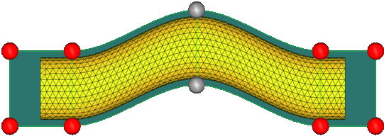
Pipe model with handles for the shapes

1.	Start HyperMesh Desktop.

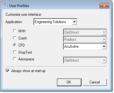
2.	In the User Profiles dialog, set the user profile to Engineering Solutions, CFD, AcuSolve.

ensol_profile

3.	From the menu bar, click File > Open > Model.

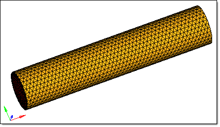
4.	In the Open Model dialog, open the pipe.hm file. A finite element model appears in the graphics area.

hs_1535_finite_element

1.	In the Model browser, right-click and select Create > Material from the context menu. A new material opens in the Entity Editor.

hs_1535_new_material

2.	In the Entity Editor:

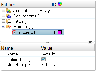
a.	For Name, enter Air_HM.

b.	Set Card Image to FLUID.

3.	Create a second material named Water_HM, and set the card image to FLUID.

4.	In the Model browser, Component folder, click inflow. The Entity Editor opens and displays the component's corresponding data.

5.	For Type, select INFLOW.

hs-1535-4

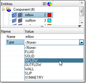
6.	Change the Type for the following components:

Component	Type
outflow	OUTFLOW
wall	WALL
fluid	FLUID

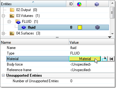
7.	In the Model browser, Components folder, click fluid. The Entity Editor opens and display's the component's corresponding data.

8.	For Material, click Unspecified >> Material.

hs-1535-5

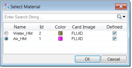
9.	In the Select Material dialog, select Air_HM and then click OK.

hs-1535-6

10.	In the Model browser, Components folder, click inflow. The Entity Editor opens and display's the component's corresponding data.

11.	For Inflow type, select Mass flux.

12.	For Mass flux ## (kg/sec), enter 0.0003.

1.	In the panel area, click HyperMorph > morph volumes.

2.	Go to the create subpanel.

3.	Activate the entity selector.

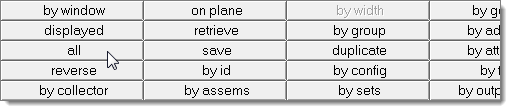
4.	Click elems > all. All of the elements in the model are selected.

create elems sub panel

5.	Click create. A new morph volume is created.

6.	Go to the split/combine subpanel.

7.	In the graphics area, double-click on the edge of the model that is marked by a green cross in the image below:

hs_1535_split

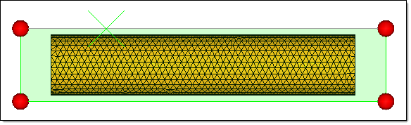
8.	Click split. The morph volume splits.

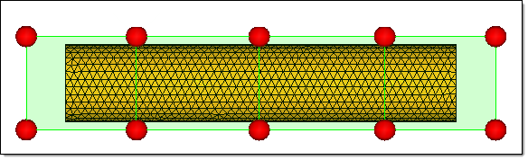
9.	Continue splitting the morph volume so that it resembles the image below.

hs_1535_split 3

10.	Go to the update edges subpanel.

11.	Click the first arrow and select update ends.

12.	Click the third arrow and select master-slave.

Note:

This options allows you to link any two edges together with a “master-slave” relationship between two morph volumes.

hs-1535-1

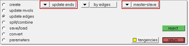
Settings for steps 3.11 and 3.12.

13.	Define the master edge by clicking the first edge of the morph volume.

14.	Define the slave edge by clicking the edge that touches the master edge.

15.	Repeat steps 3.13 and 3.14 for all of the edges until your model resembles the image below (look for yellow arrows).

hs_1535_master_slave

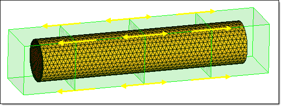
16.	Click return to go back to the HyperMorph panel.

17.	In the panel area, click morph.

18.	Go to the move handles subpanel.

19.	Click the second arrow and select translate.

20.	Under translate, click the arrow and select along vector.

21.	Under along vector, set the orientation selector to y-axis.

22.	In the dist = field, enter 0.010.

hs-1535-2

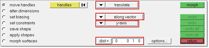
Settings for steps 3.19 through 3.22.

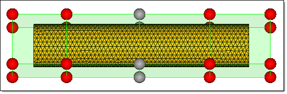
23.	Activate the handles selector.

24.	Select the four middle handles, highlighted in grey, in the image below:

hs_1535_morphgrid

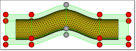
25.	Click morph. The grid is morphed.

hs_1535_morph

26.	Go to the save shape subpanel.

27.	In the name= field, enter s1.

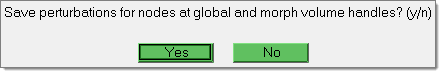
28.	Switch the first toggle from as handle perturbations to as node perturbations.

29.	Click save.

30.	In the window that appears, click Yes.

hs-1535-3

31.	Click undo all.

32.	In the Model browser, right-click on the Shape folder and select Hide from the context sensitive menu. The shape, s1 is hidden.

33.	Right-click on the Shape folder again and select Show from the context sensitive menu. The shape, sh1 reappears.

34.	From the menu bar, click View > Browsers > HyperMesh > Utility.

35.	In the Utility browser, click Disp.

36.	Remove any temporary nodes in the model by clicking Clear Temp Nodes.

37.	Create design variables by clicking Design Study > Define DV from the menu bar.

38.	Go to the desvar subpanel.

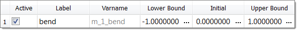
39.	In the desvar = field, enter bend.

40.	Click shape =.

41.	Link a shape with the shape design variable by clicking s1.

42.	Click create. The design variable bend is created.

43.	Click return.

1.	On the CFD toolbar, click . The HyperStudy Job Launcher opens.

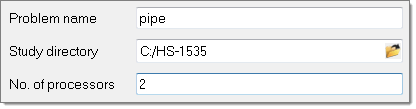
2.	In the Study directory field, navigate to the location of your working directory.

Note:

By default path will be the same directory in which the .hm file is saved. It is recommended that you create a separate folder for your study directory so that all of the files will be placed in that folder.

3.	In the No. of processors field, enter 2.

hs_1535_job_launcher1

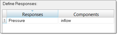
4.	In the Define Output Responses table, select the following to identify what the pressure change will be at inflow due to shape changes.

a.	Set Responses to Pressure.

b.	Set Components to inflow.

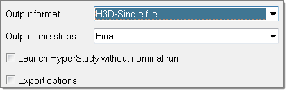
hs_1535_hst_job_launcher_define_responses

5.	To see how the pressure contours for each optimum design will look, set Output format to H3D-Single file.

hs_1535_job_launcher2

6.	Click Launch.

7.	In the dialog that opens asking if you would like to continue, click Yes.

8.	In the dialog that opens informing you of the files that were created, click OK.

9.	In the dialog that opens asking if you would like to continue, click Yes.

10.	A nominal run is submitted, and acuProbe and acuTrail are launched to provide you with updated information about the run. Once the run is finished, HyperStudy opens and with the study Setup completed.

hs-1535-10

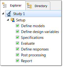
11.	Go through each step to ensure that everything was properly defined.

12.	In the Define models step, you will see that the resource file, solver input file, and solver execution script have been defined.

hs-1535-11

13.	In the Define Input Variables step, you will see that the input variable you defined in HyperMesh Desktop has been imported.

hs-1535-12

14.	In the Define Output Responses step, ensure that the output response is defined correctly.

1.	In the Explorer, right-click and select Add Approach from the context menu.

2.	In the HyperStudy - Add dialog, select Doe and click OK.

3.	Go to the Specifications step.

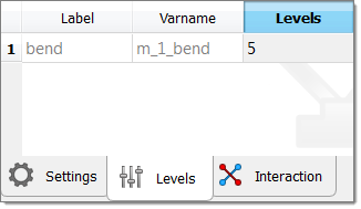
4.	In the work area, set the Mode to Full Factorial.

5.	Click the Levels tab.

6.	Change the number of levels to 5.

hs_1535_levels_column

7.	Click Apply.

8.	Go to the Evaluate step. The table used to run the study appears, showing all of the runs (1 - 5) to be executed.

9.	Click Evaluate Tasks.

10.	To view the optimization results of the five runs in a table, click the Evaluation Data tab. The table displays the results of the five runs for the output responses.

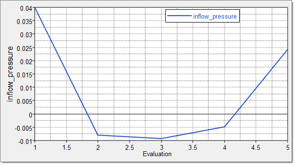
11.	To plot the optimization results of the five runs, click the Evaluation Plot tab.

Plot the results of the inflow_pressure output response by selecting inflow_pressure with the Channel selector..

hs_1535_plot

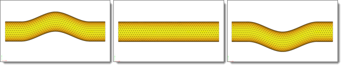
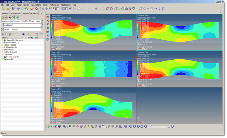
12.	The extreme left (bend = -1), middle (bend = 0) and extreme right (bend = 1) results correspond to the following pipe shapes.

hs_1535_pipe shapes

13.	Click File > Save As from the menu bar to save the study.

14.	In the HyperStudy - Select location dialog, navigate to your working directory and save the study.

15.	The results of the DOE can be visualized in HyperView. Load the corresponding *.h3d file from the run folder into HyperView.

hs_1535_hyperview

HS-1535: Coupling HyperStudy, Morphing and AcuSolve (HyperStudy Job Launcher)

HS-1535: Coupling HyperStudy, Morphing and AcuSolve (HyperStudy Job Launcher)

HS-1535: Coupling HyperStudy, Morphing and AcuSolve (HyperStudy Job Launcher)

See Also: