In this tutorial, you will learn how to perform a DOE and Optimization study of a fan using Altair HyperMesh®, Altair HyperStudy®, and ANSYS CFX®. The DOE results are used to create a response surface approximation to the fan efficiency (objective function), followed by the optimization of the blade shape using the same output response approximation.
This tutorial and the associated images were created on Windows, however all steps are identical on UNIX systems, except for changes in directory paths.
The files used in this tutorial can be found in <hst.zip>/HS-1545/. Copy the tutorial files from this directory to your working directory. The tutorial directory includes the following files:
fan_6_blades.hm -
|
HyperMesh file: (1/6) of the six-blade fan model.
|
HST_CFX.tcl -
|
Customizable execution script for CFX (Windows and UNIX).
|
preferences_wish.mvw -
|
Preferences file to add wish as a solver to execute HST_CFX.tcl.
|
model.pre -
|
CFX-Pre command file. Used to generate a new model.def definition file for CFX-Solve. This file can be customized to meet the specific needs of other models.
|
CFX_options.txt -
|
Customizable command line options for CFX-Solve.
|
model.cse -
|
CFX-Post session file. Used to extract the quantities of interest from CFX results files (model.res). Fan efficiency is the model output response used for optimization in this tutorial example.
|
In this tutorial, you will:
| • | Do a shape parameterization using HyperMorph and export model/shapes for HST / CFX. |
| • | Set-up a new study with HyperStudy. |
| • | Run the DOE study with HyperStudy and CFX. |
| • | Post process the DOE results and generate output response approximations with HyperStudy. |
| • | Perform a shape optimization based on the DOE results/output response approximations. |
The first step to carry out a successful DOE / optimization study is to have a sound CFX model that converges reasonably well and produces meaningful simulation results. This is a baseline model and would be a model that has already been simulated with CFX. We have generated the files model.cfx and model.res; the latter file (baseline simulation results) can be used to initialize each DOE run, thus reducing the total CPU/wall time necessary to reach convergence.
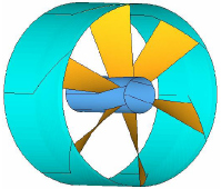
For completeness, this tutorial describes typical steps followed during an initial or baseline CFX simulation for which a file created in HyperMesh, fan_6_blades.hm, will be used.
After performing the baseline simulation, a DOE study will be done to examine how fan efficiency depends on changes in the blade geometry at constant RPM and flow rate. These operating conditions (boundary conditions) are selected because CFX converges very quickly. Efficiency will be measured as the ratio between the power transferred to the airflow and the mechanical power consumed by the rotating blades. This is just one illustrative example among the many types of studies that can be done using CFX with HyperMesh and HyperStudy.
| 1. | Start HyperMesh Desktop. |
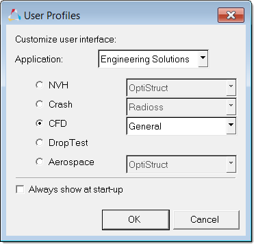
| 2. | In the User Profiles dialog, select Engineering Solutions, CFD, General. |
| 4. | From the menu bar, click File > Open > Model. |
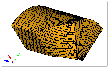
| 5. | In the Open Model dialog, open the fan_6_blades.hm file. A finite element model appears in the graphics area. |
| Note: | This model's mesh contains 3D elements in the fluid_rot component, and 2D elements (for boundary conditions) in the remaining components. |
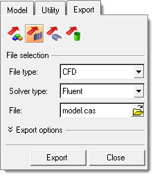
| 6. | From the menu bar, click File > Export > Solver Deck. |
| 8. | Set Solver type to Fluent. |
| 9. | In the File field, save the file as model.cas. |
| 11. | In the first dialog that opens, asking if you would like to continue, click Yes. |
| 12. | In the second dialog that opens, informing you that the model.cas file was created, click OK. |
|
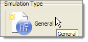
| 3. | From the menu bar, click File > New Simulation. |
| 4. | In the Simulation Type area, click General. |
| 6. | In the dialog that opens, click OK. |
| 7. | From the menu bar, click File > Import Mesh. |
| 8. | From the File type list, select Fluent (*cas). |
| 9. | Navigate to your working directory and open the model.cas file. |
| Note: | The default mesh units should not change “m.” |
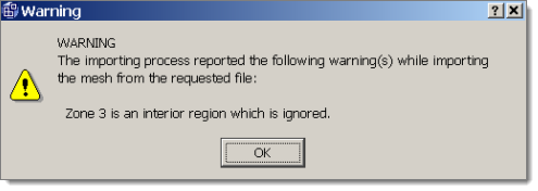
| 10. | If a Warning dialog opens, click OK. |
| Note: | This is fine, as it is referring to the way FLUENT CAS files define the meshes by internal faces. |
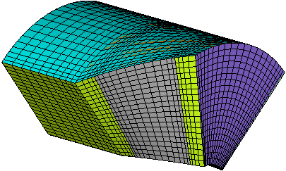
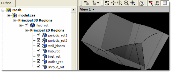
| 11. | The mesh with all boundary conditions will be read and displayed as shown in the image below. |
| Note: | All boundary components have been read with exactly the same names used in HyperMesh. |
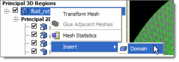
| 12. | From the Principle 3D Regions list, right-click on fluid_rot and select Insert > Domain from the context sensitive menu. |
| 13. | Under Domain Motion, change the Option to Rotating. |
| 14. | In the Angular Velocity field, enter 2000 rev min^-1. |
| 15. | Leave the default Rotation Axis of Global Z. |
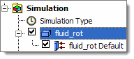
| 17. | In the Simulation folder, double-click on Simulation > fluid_rot to open the Domain: fluid_rot tab and inspect the associated values. |
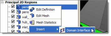
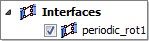
| 18. | From the Principle 2D Regions list, right-click on Principal 2D Region, periodic_rot1 and select Insert > Domain Interface from the context sensitive menu. |
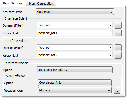
| 19. | In the Domain interface definition tab, define the rotational periodicity interface as indicated in the image below. |
| 20. | A new domain interface will be visible. |
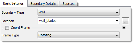
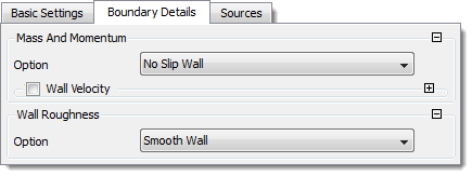
| 21. | From the Principle 2D Regions list, right-click on wall_blades and select Insert > Boundary > Wall from the context sensitive menu. |
| 22. | In the Boundary: wall_blades dialog, select the parameters indicated in the images below. |
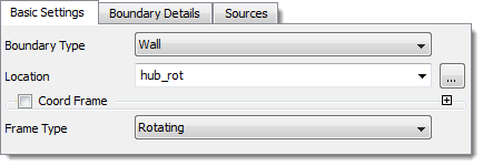
| 24. | Right-click on hub_rot and select Insert > Boundary > Wall from the context sensitive menu. |
| 25. | In the Boundary: hub_rot dialog, select the parameters indicated in the images below. |
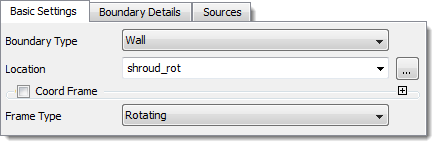
| 27. | Right-click on shroud_rot and select Insert > Boundary > Wall from the context sensitive menu. |
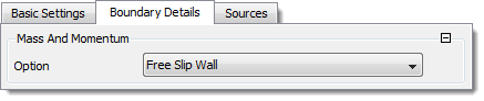
| 28. | In the Boundary: shroud_rot dialog, select the parameters indicated in the images below. |

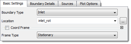
| 30. | Right-click on inlet_rot and select Insert > Boundary > Inlet from the context sensitive menu. |
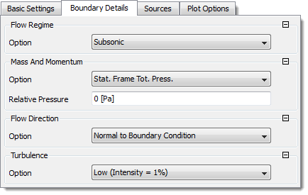
| 31. | In the Boundary: inlet_rot dialog, select the parameters indicated in the images below. |
| 33. | Right-click on outlet_rot and select Insert > Boundary > Outlet from the context sensitive menu. |
| 34. | In the Boundary: outlet_rot dialog, select the parameters indicated in the images below. |
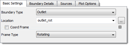
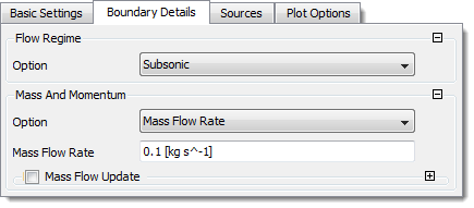
| 35. | Click OK. The boundary conditions to analyze the performance of this fan under constant air flow rate and rotor RPM are now defined. |
| 36. | To save the CFD simulation model, click File > Save Case As from the menu bar. |
| 37. | Navigate to your working directory and save the file as model.cfx. |
| 38. | To write the solver file, click Tool > Solve > Start Solver and Monitor from the menu bar. |
| 39. | In the Write Solver Input File dialog, navigate to your working directory and save the file as model.def. |
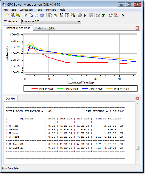
| 40. | In the CFX-Solver Manager dialog, the solver will converge in approximately 45 iterations. |
| 41. | If the CFX-Solver Manager dialog appears, click Post Process Results; if the dialog does not appear start CFD-Post and load the .res file created by the CFX Solver. |
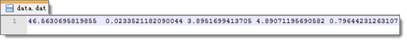
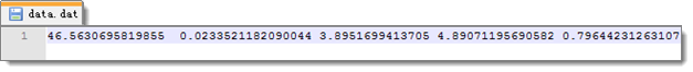
| 42. | Review the user-customizable CFX-Post session file model.cse, which defines several performance parameters and saves them to a file named data.dat. |
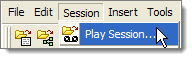
| 43. | To execute this session file, click Session > Play Session from the menu bar. |
| 44. | Navigate to your working directory and open the model.cse file. After a couple of seconds, a new file named data.dat will be available in your working directory. The file data.dat (shown below) has five columns, a description of each column value can be found browsing model.cse. The rightmost column with value 0.796. is the fan efficiency calculated as the ratio between the power transferred to the airflow (outlet – inlet) and the mechanical power consumed by the rotating blades. |
CFX-Solve saves results files with the name model_###.res, where ### represents a version number. Very often it is advisable to initialize the simulations done in the DOE with this baseline results file to decrease total run time. For this reason, it is advisable to rename a good baseline results file model_###.res to model.res, and use this name in file CFX_options.txt (inspect the contents of this file which depends on your solution approach, hardware, etc). The file CFX_options.txt contains the command line options that are passed to the CFX solver in each of the runs started by HyperStudy.
| 45. | Exit all CFX tools (e.g. Pre, Solve, Post) so that the license is available for the HyperStudy DOE/optimization runs. Now you can begin generating the blade’s optimization shapes/parameterization in HyperMesh using this model. |
|
| 1. | Optional: If you closed your previous Engineering Solutions session with the fan_6_blades.hm model, reopen it. |
| 2. | In the Model browser, Component folder, right-click on fluid_rot and select Isolate Only from the context menu. All of the components are hidden in the graphics area, except fluid_rot. |
| 3. | In the panel area, click HyperMorph. |
| 4. | Click domains. The Domains subpanel opens, from which you can create domains for the shape parameterization. |
| Note: | For this tutorial, you can use the domains that are generated automatically. |
| 5. | Go to the create subpanel. |
| 6. | Click the first arrow and select 3D domains from the list. |
| 7. | Switch the toggle from all elements to elems. |
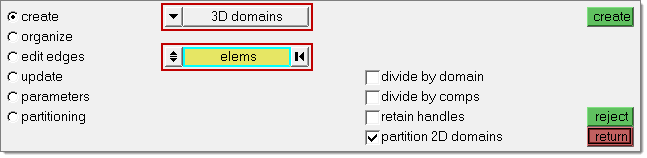
Settings for steps 3.6 and 3.7.
| 8. | On the Standard Views toolbar, click  . The graphics area displays the XZ Right Plane View of the model. . The graphics area displays the XZ Right Plane View of the model. |
| 9. | To rotate the model view clockwise 90 degrees, click  on the Standard Views toolbar. on the Standard Views toolbar. |
| Note: | The model's X-Axis should point upwards and the Z-Axis should be point to the right, as indicated in the following image. |
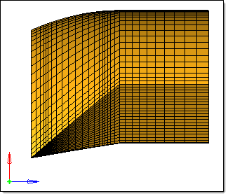
| 10. | Select all of the elements on the left half of the model. |
| Tip: | Use box selection to quickly select elements. To box select, press SHIFT while left-clicking, then drag your mouse. |
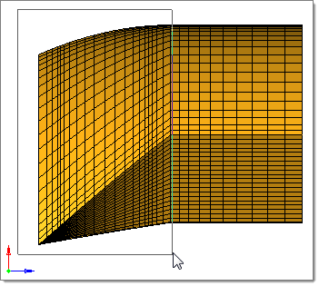
| 11. | Click create. A 3D domain and handles are created in the model. |
| 12. | Go to the parameters subpanel. |
| 13. | In the handle size= field, enter 0.005. |
| 14. | Click return. It make take a couple of seconds to regenerate the data structure before you are returned to the HyperMorph panel. |
| 15. | Click morph. The Morph subpanel opens, from which you can morph the shape of the mesh. |
| Note: | The objective of the following steps is to create two input variables. The first input variable will change the blades angle, and the second input variable will change the fan thickness. |
| 16. | Go to the move handles subpanel. |
| 17. | Click the first arrow and select handles. |
| 18. | Select the four handles on the fan inlet face of the model. |
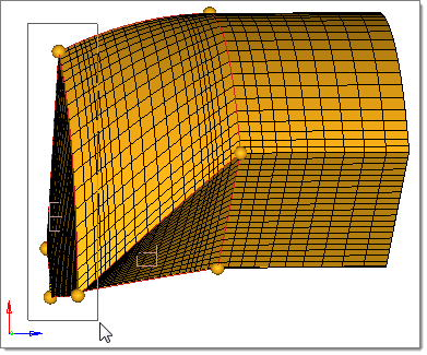
| 19. | Click the second arrow and select rotate. |
| 20. | Select the true rotation checkbox. |
| 21. | Under rotation axis, select z-axis. |
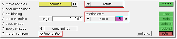
Settings for steps 3.19 through 3.21.
| 22. | To select the base point for rotation, click  . . |
| 23. | In the x=, y= and z= fields, enter 0.0. |
| 25. | In the angle field, enter 5.0 (degrees). |
| 26. | Click morph. The first shape is generated. |
| 27. | Go to the save shape subpanel. |
| 28. | Switch the first toggle from as handle perturbations to as node perturbations. |
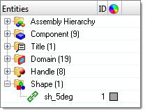
| 29. | In the name= field, enter sh_5deg. |
| 30. | Click save. The new shape appears in the Model browser. |
| 31. | To prepare for the generation of the next shape, click undo all. |
| 32. | Go to the move handles subpanel. |
| 33. | Repeat steps 17 and 18 above. |
| 34. | Click the first arrow and select Translate. |
| 35. | Click the second arrow and select along xyz. |
| 36. | In the z val= field, enter 0.005. |
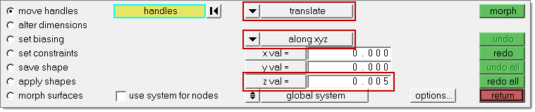
Settings for steps 3.34 through 3.36.
| 37. | Click morph. A second shape is generated. |
| 38. | Go to the save shape subpanel. |
| 39. | Switch the first toggle from as handle perturbations to as node perturbations. |
| 40. | In the name= field, enter sh_5mm. |
| 41. | Click save. The new shape appears in the Model browser |
|
| 1. | In the panel area, click shape. |
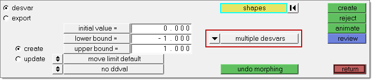
| 2. | Go to the desvar subpanel. |
| 3. | Click the first arrow and select multiple desvars. |
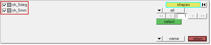
| 5. | Select the shapes sh_5deg and sh_5mm. |
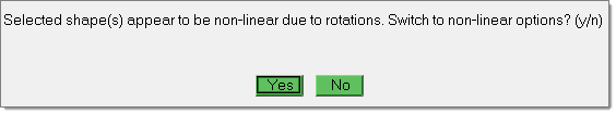
| 8. | In the window that appears, asking if you would like to switch to non-linear options, click No. An input variable is created for each shape selected. |
| 9. | Optional: If you would like to animate or visualize the shapes, click animate. |
| 10. | Optional: In the Deformed panel, click linear or modal to animate the shape variables in the graphics area. |
| 11. | Optional: While the shape is animating, you can adjust the animation speed by moving the slider as indicated in the following image. |
| 12. | To exit the panels, click return. |
| 13. | From the menu bar, click File > Save As > Model. |
| 14. | In the Save Model As dialog, save the file as fan_6_blades_2shapes.hm. |
| 15. | From the menu bar, click View > Browsers > HyperMesh > Utility. |
| 16. | In the Utility menu, click CFD I/O. |
| 17. | Under Export files for CFX, click Shapes. |
| 18. | In the dialog that appears, asking if you would like to continue, click Yes. |
| 19. | In the Open baseline ACSII case file dialog, open the model.cas file. |
| 20. | In the dialog that appears, alerting you that your files have finished writing, click OK. |
| 21. | In the dialog that appears, alerting you that the HyperStudy template file for Fluent has been created, click OK. The following files are created: |
model.shp Grid perturbation vector data read by file model.fluent.node.tpl.
model.fluent.node.tpl Grid coordinates template.
model.tpl Fluent case template read by HyperStudy.
|
| 2. | Register the WISH interpreter as a solver to run the CFX simulation. |
| a. | From the menu bar, click File > Use Preferences File. |
| b. | In the HyperStudy - Set Preference File dialog, open the preference_wish.mvw file. |
| 3. | To start a new study, click File > New from the menu bar, or click  on the toolbar. on the toolbar. |
| 4. | In the HyperStudy – Add dialog, enter a study name, select a location for the study, and click OK. |
| Note: | It is important that you select the study directory that contains all the files that you generated earlier. These files include the CFX native files: model.cfx, model.pre, model.cse, and (if you plan to customize your CFX solution with command line arguments) CFX_options.txt. If you are restarting from an existing .res file, make sure the model.res file is also in your study directory. |
For advanced users: The CFX_options.txt file can be changed at any time while HyperStudy is running. This file is copied to the execution directories (e.g. m_1) at the time when the simulation in that particular directory is starts, not when HyperStudy first writes the .cas file to that directory. Verify that the options are correct, otherwise CFX-Solve will abort the run. A typical use could be to add a command line option to run in parallel, use a lower priority, etc.
| 5. | Go to the Define models step. |
| 6. | Add a Parameterized File model. |
| a. | From the Directory, drag-and-drop the model.tpl file into the work area. |
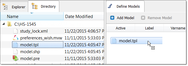
| b. | In the Solver input file column, enter model.cas. This is the name of the solver input file HyperStudy writes during any evaluation. |
| c. | In the Solver execution script column, select Wish (wish). |
| d. | In the Solver input arguments column, enter HST_CFX.tcl before $file. This is the name of the CFX execution script. |
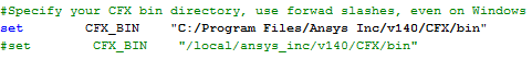
Append the absolute path to the beginning of HST_CFX.tcl. For example, C:/test/HST_CFX.tcl; on UNIX: /users/local/HST_CFX.tcl or equivalent.
Optional. If you are running HyperStudy on Linux, enter -nobg after $file. For example, /users/local/HST_CFX.tcl $file -nobg.

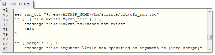
Save the HST_CFX.tcl file to a location that can be reused by all optimization studies. The HST_CFX.tcl file contains specific information about the CFX installation directory, as illustrated in the image below.
| Note: | The optional CFX_options.txt file contains command line options that are passed to the CFX solver in each of the runs started by HyperStudy. Inspect the contents of this file. The contents will vary depending on your solution approach, hardware, and so on. Comment lines start with #, and the last defined “CFX_OPTS =” statement is used. One of the main functions of this file is to specify an initialization results file. The objective is to speed up the convergence of each run by initializing the solution with the results from the baseline run done before starting the DOE/optimization work. It is crucial to make sure that the .res file specified exists, and that the path name is correct. |
| 7. | Rename your baseline results file mode_###.res to model.res so that the file name listed after -ini exists. |
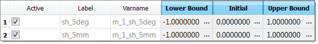
| 8. | Click Import Variables. Two input variables are imported from the model.tpl file. |
| 9. | Go to the Define Input Variables step. |
| 10. | Review the input variable's lower and upper bound ranges. |
| 11. | Go to the Specifications step. |
|
| 1. | In the work area, set the Mode to Nominal Run. |
| 3. | Go to the Evaluate step. |
| 4. | Click Evaluate Tasks. An approaches/nom_1/ directory is created inside the study directory. This directory contains the model.cas file, which is the input mesh file generated by HyperStudy, and the CFX_run.log file, which is a log of HyperStudy’s scripts execution (read the contents of this file if there are any errors). The approaches/nom_1/run__00001/m_1 directory contains the pre_script.bat.out, solve_script.bat.out, and post_script.bat.out files, which are the output files from the CFX’s Pre, Solve, and Post executables. These file will contain information regarding any licensing or runtime problems that may have occurred. If everything is correct, you will find the data.dat file specified as output in your model.cse file; this file contains five columns as described previously. |
| 5. | Go to the Define Output Responses step. |
|
In this step you will create three output responses: Efficiency, W_fluid, W_blades.
| 1. | Create the Efficiency output response. |
| a. | From the Directory, drag-and-drop the data.dat file, located in the approaches/nom_1/run__00001/m_1 directory, into the work area. |
| b. | In the File Assistant dialog, set the Reading technology to Altair® HyperWorks® and click Next. |
| c. | Select Single item in a time series, then click Next. |
| d. | Define the following options, and then click Next. |
| • | Set Component to Column 5. |
| e. | Label the output response Efficiency. |
| f. | Set Expression to First Element. |
| Note: | This expression evaluates the fifth column of the first (and only) line of file data.dat. |
| g. | Click Finish. The Efficiency output response is added to the work area. |
| 2. | Repeat step 1 to create the output responses W_fluid and W_blades. |
| • | For W_fluid, set Component to Column 3. |
| • | For W_blades, set Component to Column 4. |
| 3. | Click Evaluate Expressions to extract output response values. |
|
| 1. | In the Explorer, right-click and select Add Approach from the context menu. |
| 2. | In the HyperStudy - Add dialog, select Doe and click OK. |
| 3. | Go to the Select Input Variables step. |
| 4. | Verify that the input variable's Lower Bound, Initial and Upper Bound values are -1.0, 0.0, 1.0. |
| 5. | Go to the Specifications step. |
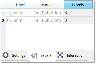
| 6. | In the work area, set the Mode to Full Factorial. |
| 8. | Change the number of levels for both input variables to 3. |
| 10. | Go to the Evaluate step. |
| 11. | Click Evaluate Tasks to start solving the run matrix. |
| 12. | Go to the Post processing step. |
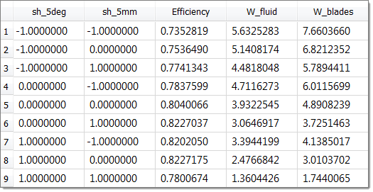
| 13. | Click the Summary tab to view a table of all of the output responses extracted from the nine runs. |
The lowest average inlet pressure occurs during run nine, where sh_5deg and sh_5mm equal 1.0. These results make sense because the elbow has the maximum cross sectional area. The next two lowest values occur during runs six and eight, when one of the shapes has a value 1.0 and the other has a value of 0.0. In relative terms, the pressure drop for runs six and eight are not much larger than run nine.
| 14. | Click the Interaction tab to view the effects of the input variables on an output response. |
Use the Channel selector to select the following output responses: sh_5deg and sh_5mm on the Efficiency. The interactions between the output responses are plotted.
|
| 1. | In the Explorer, right-click and select Add Approach from the context menu. |
| 2. | In HyperStudy - Add dialog, select Fit and click OK. |
| 3. | Go to the Select matrices step. |
| 5. | In the HyperStudy - Add dialog, add one matrix. |
| 6. | In the Matrix Source column, select Doe 1 (doe_1). |
| 7. | Click Import Matrix. The data from Doe 1 is imported to the current Fit approach as an input matrix. |
| 8. | Go to the Specifications step. |
| 9. | In the work area, set the Mode to Least Squares Regression (LSR). |
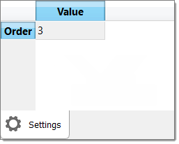
| 10. | In the Settings tab, change the Order to 3. |
| 11. | Optional. View the input matrix by clicking Edit > Run Matrix from the top, right corner of the work area. |
| 12. | Click the Regression Terms tab. |
| 13. | Using the Channel selector, select the output response Efficiency. |
| 14. | In the Active column, clear the a6 and a7 checkboxes. |
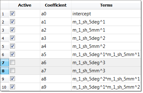
| 15. | Clear the a6 and a7 checkboxes for the output responses W_fluid and W_blades. |
| Note: | The number of sampling points is nine, but the 3rd order approximation model terms are 10. To build an approximation model with good fit quality and limited sampling points, you need to neglect the pure 3rd order terms, and keep the rest as a compromise. Later on in this tutorial, you will check the residuals and diagnostics of the fit quality for this decision. |
| 17. | Go to the Evaluate step. |
| 18. | Click Evaluate Tasks. HyperStudy computes the regression surface. |
| 19. | Go to the Post processing step. |
| 20. | Click the Residuals tab to review the residuals of fitting. |
The maximum errors are small enough in a relative sense, otherwise using the approximation to conduct an optimization will not be meaningful.
| 21. | Click the Diagnostics tab to review diagnostic information, T-values, and Confidence Intervals of the regression terms. |
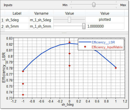
| 22. | Click the Trade-Off 2D tab to plot the response surface. |
Tune the input variables and change the curve by moving the sliders in the Value column above the plot.
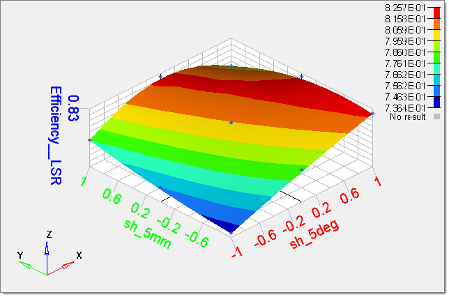
| 23. | Click the Trade-Off 3D tab to review the response surface in a 3D plot. |
|
| 1. | In the Explorer, right-click and select Add Approach from the context menu. |
| 2. | In the HyperStudy - Add dialog, select Optimization and click OK. |
| 3. | Go to the Select Input Variables step. |
| 4. | Review the input variable's lower and upper bound ranges. |
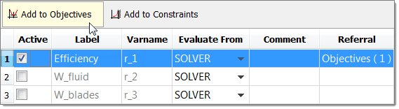
| 5. | Go to the Select Output Responses step. |
| 6. | Click the Responses tab. |
| 7. | In the Active column, clear the W_fluid and W_blades checkboxes. The Optimization will not have to rely on the CFX solution anymore. |
| 8. | Select the output response Efficiency by highlighting it in the work area. |
| 9. | Click Add to Objectives. HyperStudy creates an objective for the output response. |
| 10. | Click the Objectives tab. |
| b. | Set Evaluate From to Efficiency_LSR (r_1_fit_1). |
| Note: | You are instructed to select the Efficiency_LSR (r_1_fit_1) option rather then the Solver option, due to the fact that it will run much faster. CFD analyses generally take a considerable amount of CPU time. If you use the Solver option, a new CFX solution will need to be computed for every iteration in the optimization process, which translates to long run times. |

| 13. | Go to the Specifications step. |
| 14. | In the work area, set the Mode to Global Response Surface Method (GRSM). |
| 16. | Go to the Evaluate step. |
| 17. | Click Evaluate Tasks to start the Optimization. |
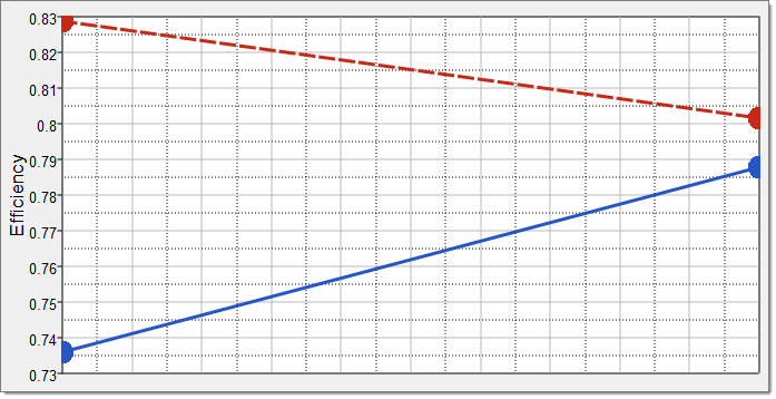
| 18. | Click the Iteration Plot tab to plot the iteration history of the objectives, constraints, input variables, and unused output responses. |
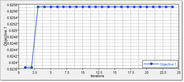
| 19. | Click the Iteration History tab to review the actual values of the input variables and the associated values of all the output responses for every iteration in the optimization process. The green rows represent the optimal designs throughout the iteration history. The best design was found in iteration 4. No better design is found in the subsequent iterations which indicates that this design is likely not a poor local minimum. |
The main objective of this optimization study was to illustrate the steps involved in doing a shape optimization based on the results of a Doe study and associated approximations. The maximum efficiency was obtained optimizing a response surface approximation. It is recommended that such predictions be verified by running a small DOE study zooming in on a small sub-domain (of the whole design space) around the optimum design found through the optimization of the global approximation. Doing so will verify (with the CFX solver) that the optimized design actually delivers the performance expected.
|
This tutorial illustrated the main steps to perform a DOE study, to build an approximation from the DOE results, and to perform a shape optimization study based on a Least Square Regression approximation. HyperMesh was used to generate the mesh for CFX and the shape variables used to modify the geometry of the fan model. HyperStudy and CFX were used to perform the DOE and optimization studies. Relatively simple modeling assumptions were used in this tutorial to minimize run times; however the steps followed in this tutorial are equally applicable to CFD optimization studies of any size and complexity.
|
See Also:
HyperStudy Tutorials


