| 1. | Open FLUENT (3ddp) Mode (Full Simulation). |
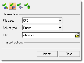
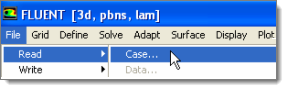
| 2. | From the menu bar, click File > Read > Case. |
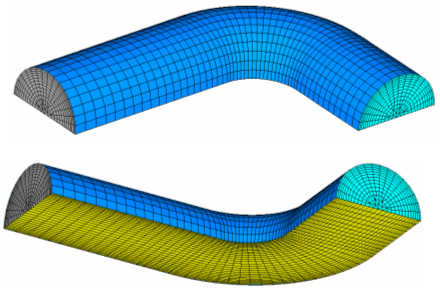
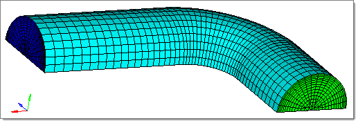
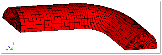
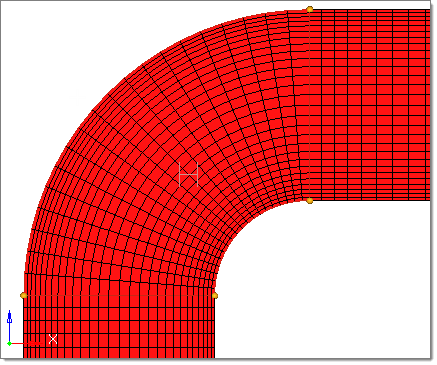
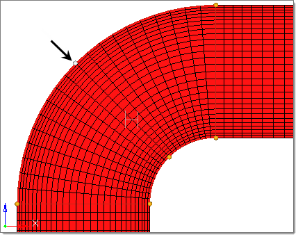
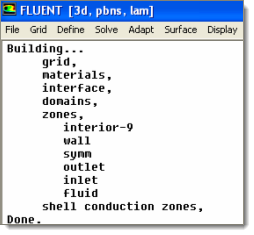
| 3. | Navigate to your working directory and open the elbow.cas file. FLUENT reads the mesh (with all boundary conditions) as illustrated below: |
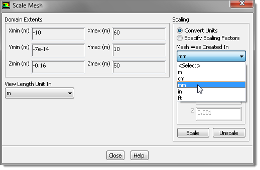
| 4. | HyperMesh Desktop created the mesh in mm length units. In order to define the simulation you need to scale the mesh to the correct dimensions first by clicking Mesh > Scale from the menu bar. |
| 5. | In the Scale Mesh dialog, click Convert Units. |
| 6. | From the Mesh Was Created In list, select mm. |
| 7. | Click Scale. FLUENT scales the dimensions to the mm unit. |
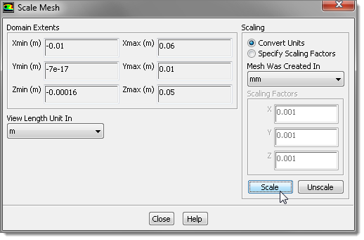
| 8. | Click Close. You can leave all of the default options for fluid (air), viscous model (Laminar), and so on. |
| 9. | From the menu bar, click Define > Boundary Conditions. |
| 10. | In the Zone area, click inlet. |
| 11. | From the Type list, select mass-flow-inlet. |
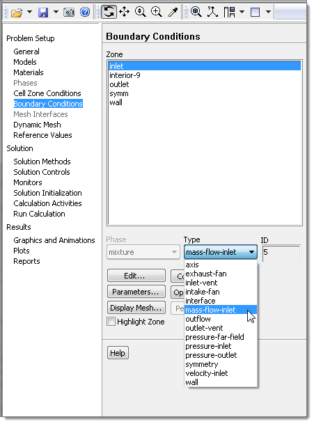
| 12. | In the dialog that appears prompting you to change the inlet type, click Yes. |
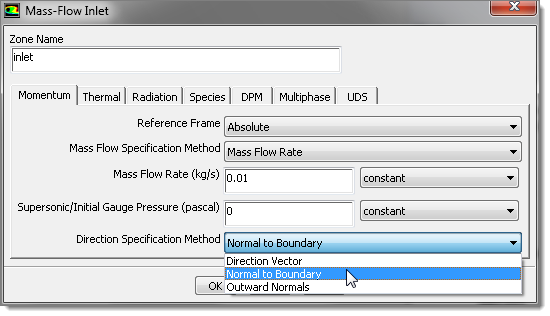
| 13. | In the Mass-Flow Inlet dialog, enter 0.01 in the Mass Flow Rate (kg/s). |
| 14. | From the Direction Specification Method list, select Normal to Boundary. |
| 16. | In the Zone area, click Outlet. |
| 17. | From the Type list, select pressure-outlet. |
| 18. | In the dialog that appears prompting you to change the outlet type, click Yes. |
| 19. | In the Pressure Outlet dialog, accept default setting of 0 Pascal and click OK. |
| 20. | Leave the symm and wall boundaries with their default values. In the Doe study, you will be monitoring the average pressure on the inlet surface. |
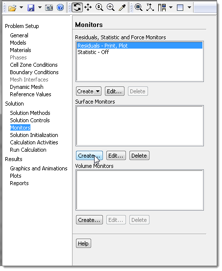
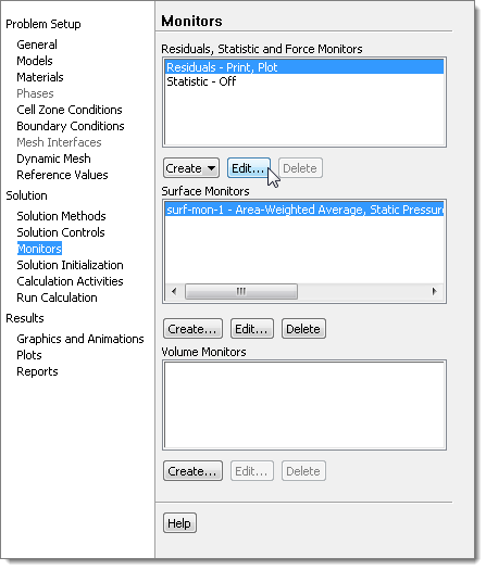
| 21. | From the menu bar, click Solve > Monitors. |
| 22. | In the Surface Monitors area, click Create. |
| 23. | In the Surface Monitors dialog, select the Plot and Write check boxes. |
| 24. | From the Report Type list, select Area-Weighted Average. |
| 25. | From the Field Variable lists, accept the default selections of Pressure and Static Pressure. |
| 26. | In the Surfaces area, select inlet. |
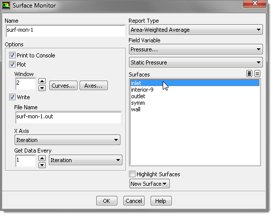
| 27. | In the File Name field, accept the default filename surf-mon-1.out. You will use this file in HyperStudy during the Doe and/or Optimization stuides. |
| Note: | For both Windows and UNIX systems, verify that that surf-mon-1.out file does not include directory information, otherwise this file will always be created in that directory. You will need the surf-mon-1.out file in the execution directories. |
| 29. | In the Residuals, Statistic and Force Monitors area, select Residuals - Print, Plot. |
| 31. | In the Residuals Monitors dialog, select the Print to Console check box. |
| 32. | In the Residual Values area, select the Normalize check box. |
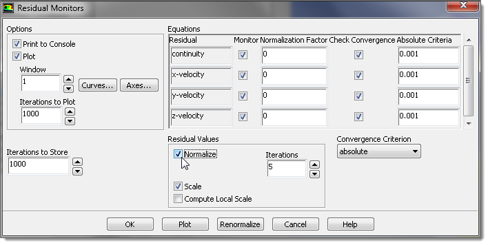
| 33. | Accept all of the other default settings and click OK. FLUENT will save the case file now. |
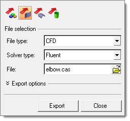
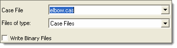
| 34. | From the menu bar, click File > Write > Case. |
| 35. | In the Case File field, enter elbow.cas. |
| 36. | Click OK (accept overwrite). You can now initialize the FLUENT simulation. |
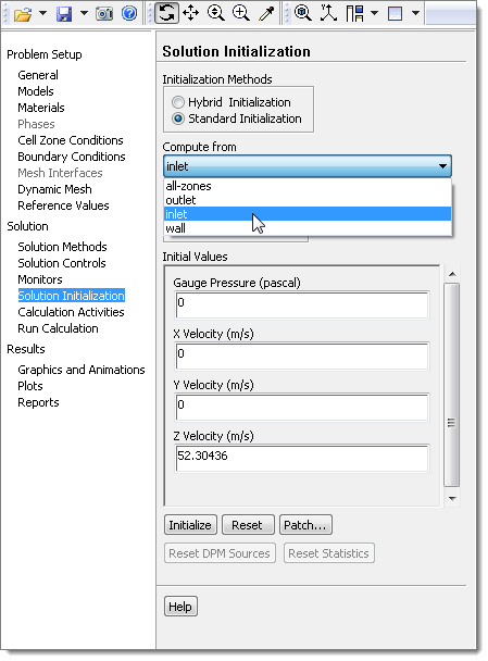
| 37. | From the menu bar, click Solve > Initialization. |
| 38. | In the Initialization Methods area, click Standard Initialization. |
| 39. | From the Compute from list, select inlet. |
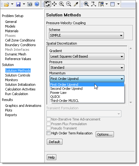
| 41. | From the menu bar, click Solve > Methods. |
| 42. | From the Momentum list, select First Order Upwind. You can now perform the baseline simulation. |
| 43. | From the menu bar, click Solve > Run Iterations. |
| 44. | In the Number of Iterations field, enter 1000. |
| 45. | Click Calculate. The solution converges to ~ 100 - 160 iterations depending on the solver version. The maximum air velocity is approx 85 m/s. |
| 46. | From the menu bar, click Report > Surface Integrals. |
| 47. | Click Report Type Area-Weighted Average. |
| 48. | Accept the defaults settings in the Field Variable area for Pressure and Static Pressure. |
| 49. | For Surfaces, select inlet. |
| 50. | Click Compute. FLUENT prints the value (approx.) 408.63 Pa. The same value appears on the last line of file surf-mon-1.out in the current directory. |
| 51. | To save the solution, click File > Write > Data from the menu bar. |
| 52. | Accept the default file name Elbow.dat and click OK. |
| 53. | To save the case file, click File > Write > Case from the menu bar. |
| 54. | Accept the default file name Elbow.cas. |
| 55. | Clear the Write Binary Files check box. |
| 56. | Click OK. You do not want to write a binary case file because you will need to read the case file while doing the Doe and/or Optimization studies. |
| 57. | Exit FLUENT. You are now ready to import elbow.cas file into HyperMesh, and create the shape design variables (geometrical changes) that will be used for the Doe and/or Optimization stuidies. |
|