This tutorial demonstrates how to run a DOE study on simple functions defined using a Templex template.
The base input template defines two input variables; DV1 and DV2, labeled X and Y, respectively. The objective of the study is to investigate the two input variables X, Y forming the two functions: X+Y and 1/X + 1/Y – 2.
Before running this tutorial, you must complete tutorial HS-1700: Simple DOE Study or you can import the archive file HS-1700.hstx, available in <hst.zip>/HS-1705/.
| 1. | In the Explorer, right-click and select Add Approach from the context menu. |
| 2. | In the HyperStudy - Add dialog, select Doe and click OK. |
| 3. | Go to the Specifications step. |
| 4. | In the work area, set the Mode to Hammersley. |
| 6. | Go to the Evaluate step. |
| 7. | Click Evaluate Tasks. The evaluation results display in the work area. |
| 8. | Go to the Post processing step. |
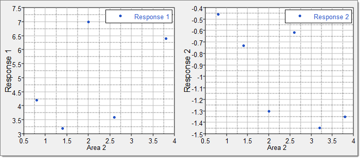
| 9. | Click the Scatter 2D tab to view a plot which illustrates the dependency between Area 2 and Response 1 and Response 2. |
| a. | Using the Channel selector, set the X Axis to Area 2 and the Y Axis to both Response 1 and Response 2. |
| b. | Compare the scatter plots to determine if the runs are distributed homogeneously throughout the design space. |
|
| 1. | In the Explorer, right-click and select Add Approach from the context menu. |
| 1. | In the HyperStudy - Add dialog, select Fit and click OK. |
| 2. | Go to the Select matrices step. |
| 4. | In the HyperStudy - Add dialog, add one matrix. |
| 5. | In the work area, set Matrix Source to Doe 2 (doe_2). |

| 7. | Go to the Specifications step. |
| 8. | In the work area, set the Mode to Least Squares Regression (LSR). |
| 10. | Go to the Evaluate step. |
| 12. | Go to the Post processing step. |
| 13. | Click the Residuals tab to review the residuals of both output responses. |
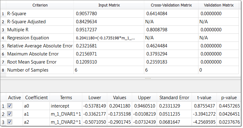
The data in the table shows the differences in the actual values and the predictions from the constructed Fit. The Percent Error column of Response_1 is numerically zero for all six runs; whereas the Percent Error column of Response_2 is up to 35%. The LSR fitting for Response_1 is acceptable, but the LSR fitting for Response_2 is rather large.
| 14. | Click the Diagnostics tab to review the overall Fit quality. |
Several measures are shown to indicate the relative quality of the Fit. The R-Square value can be interpreted as the percentage of variance in the data that can be explained by the Fit. For Response_1, the Fit captures 100% of the data variance; this makes sense as Response_1 is actually a linear function so the first order regression matches the actual data with no error. For Response_2, it is shown below that the Fit explains about 90% of the variance.
| 15. | With first order least squares, you have a Fit which explains most of the data’s variance, but it still has a relatively high prediction error. Go back to the Specifications step and try different methods until you find an acceptable fitting for both output responses. |
|
See Also:
HyperStudy Tutorials


