This tutorial demonstrates how to optimize a simple function defined using a Templex template. The base input template defines two input variables, DV1 and DV2, labeled X and Y, respectively. The objective of the optimization is to minimize X + Y with the constraint 1/X + 1/Y – 2 < 0.
Before running this tutorial, you must complete tutorial HS-1010: Simple DOE Study (or HS-1700: Simple DOE Study, HS-1705: Simple Fit Study) or you can import the archive file HS-1705.hstx, available in <hst.zip>/HS-1710/.
| 1. | In the Explorer, right-click and select Add Approach from the context menu. |
| 2. | In the HyperStudy - Add dialog, select Optimization and click OK. |
| 3. | Go to the Select Input Variables step. |
| 4. | Review the input variable's lower and upper bound ranges. |
| 5. | Go to the Select Output Responses step. |
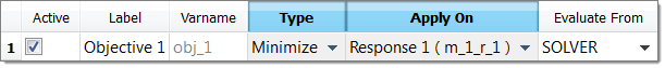
| 7. | In the HyperStudy - Add dialog, add one objective. |
| b. | Set Apply On to Response 1 (r_1). |
| 9. | Click the Constraint tab. |
| 11. | In the HyperStudy - Add dialog, add one constraint. |
| 12. | Define the constraint. |
| a. | Set Apply On to Response 2 (r_2). |
| b. | Set Bound Type to <= (greater than or equal to). |
| c. | In the Bound Value column, enter 0.0. |

| 14. | Go to the Specifications step. |
| 15. | In the work area, set the Mode to Adaptive Response Surface Method (ARSM). |
| Note: | Only the methods that are valid for the problem formulation are enabled. |
| 17. | Go to the Evaluate step. |
| 19. | Optional. Click the different tabs in the Evaluate step to monitor the progress of the Optimization. |
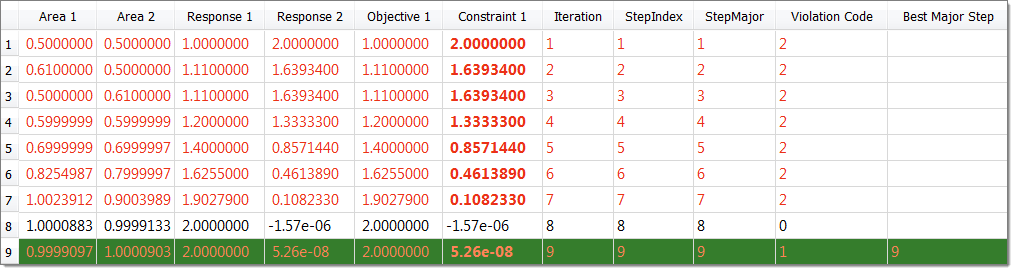
| 20. | After the optimization has finished, review the optimization history first. |
| 21. | With many of the algorithms (SQP, GA, …), each iteration requires many evaluations. |
| • | Evaluation (plots or tables) show all runs performed during the optimization. |
| • | Iteration (plots or tables) show the optimization iterations. |
The Iteration History tab uses color coding to indicate which design are feasible, optimal, and violated.
| • | White background/black font indicates the design is feasible. |
| • | White background/red font indicates the design is violated. |
| • | White background/orange font indicates the design is acceptable, but at least one constraint is near violated. |
| • | Green background/white font indicates the design is optimal. |
| • | Green background/orange font indicates the design is optimal, but at least one constraint is near violated. |
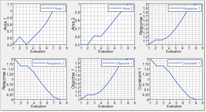
| 22. | The Evaluation Plot tab displays charts for all of the entities in the optimization (input variables, output responses, objective functions, constraints) against the iteration. |
| • | Select entities to plot using the Channel selector in the left pane. |
| • | Plot multiple entities in separate windows by clicking  . . |
| 23. | Go to the Post processing step. |
|
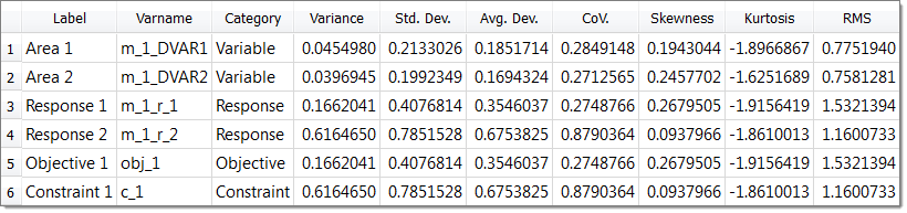
In the Post processing step of an Optimization approach, you can access additional tools to review the results. Use the Integrity, Distribution, and Scatter 2D/3D tabs to compare and analyze designs.
| 1. | Click the Integrity tab to analyze statistics of the optimization study. |
|
See Also:
HS-1700: Simple DOE Study
HyperStudy Tutorials


