This tutorial demonstrates how to perform a multi-disciplinary size optimization for two finite element models defined for OptiStruct that have common input variables. The sample base input templates plate1.tpl and plate2.tpl, can be found in <hst.zip>/HS-4210/ and copied to your working directory.
The objective is to minimize the volume of the plate under a stress and a frequency constraint. The input variables are the thickness of each of the three components, defined in the input deck via the PSHELL card. The thickness should be between 0.05 and 0.15; the initial thickness is 0.1 (shown below). The optimization type is size. To demonstrate the use of the optimization tool in a multi-disciplinary optimization, two models are created. One model is used for the stress analysis and one for the frequency analysis. Both models must have the same input variables.
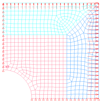
Figure 1. Double symmetric plate model.
| 2. | To start a new study, click File > New from the menu bar, or click  on the toolbar. on the toolbar. |
| 3. | In the HyperStudy – Add dialog, enter a study name, select a location for the study, and click OK. |
| 4. | Go to the Define models step. |
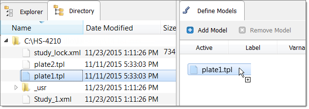
| 5. | Add a Parameterized File model. |
| a. | From the Directory, drag-and-drop the plate1.tpl file into the work area. |
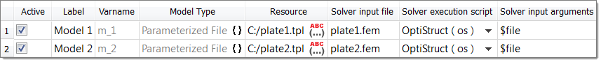
| b. | In the Solver input file column, enter plate1.fem. This is the name of the solver input file HyperStudy writes during any evaluation. |
| c. | In the Solver execution script column, select OptiStruct (os). |
| 6. | Add a Parameterized File model. |
| a. | From the Directory, drag-and-drop the plate2.tpl file into the work area. |
| b. | In the Solver input file column, enter plate2.fem. This is the name of the solver input file HyperStudy writes during any evaluation. |
| c. | In the Solver execution script column, select OptiStruct (os). |
| 7. | Click Import Variables. Six input variables are imported from the plate1.tpl and plate2.tpl resource files. |
| 8. | Go to the Define Input Variables step. |
| 9. | Review the input variable's lower and upper bound ranges. |
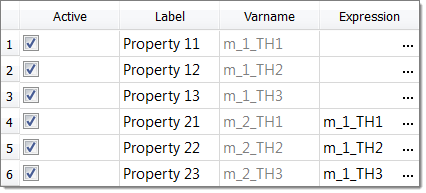
| 10. | Click the Link Variables tab. |
| 11. | In the Expression column of the input variable Property 21, click  . . |
| 12. | In the Expression Builder, click the Design Variables tab. |
| 13. | In the work area, select Property 11. |
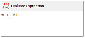
| 14. | Click Insert Varname. The expression m_1_TH1 appears in the Evaluate expression field. |
| 15. | Click OK. Property 21 of Model 2 is linked to Property 11 of Model 1. |
| 16. | Create two more links. |
| • | Link Property 22 to Property 12. |
| • | Link Property 23 to Property 13. |
| 17. | Go to the Specifications step. |
|
| 1. | In the work area, set the Mode to Nominal Run. |
| 3. | Go to the Evaluate step. |
| 4. | Click Evaluate Tasks. An approaches/nom_1/ directory is created inside the study directory. The approaches/nom_1/run__00001/m_1 and approaches/nom_1/run__00001/m_2 sub-directories contain the plate2.out (for the structural volume and frequency) and plate1.h3d (for the stresses) files, which are the results of the nominal run, and will be using during the Optimization. |
| 5. | Go to the Define Output Response step. |
|
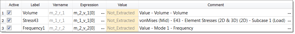
In this step you will create three output responses: Volume, Stress43, and Frequency1.
| 1. | Create the Volume output response, which represents the volume of the plate. |
| a. | From the Directory, drag-and-drop the plate2.out file, located in the approaches/nom_1/run__00001/m_2 directory, into the work area. |
| b. | In the File Assistant dialog, set the Reading technology to Altair® HyperWorks® and click Next. |
| c. | Select Single item in a time series, then click Next. |
| d. | Define the following options, then click Next. |
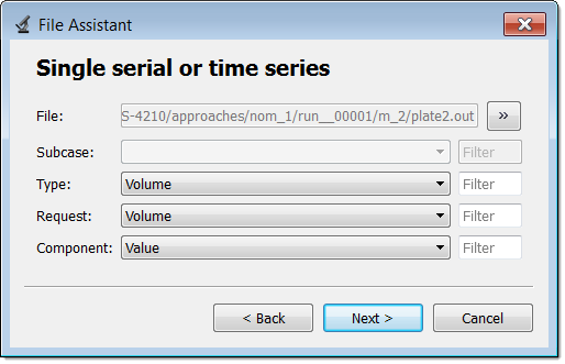
| e. | Label the output response Volume. |
| f. | Set Expression to First Element. |
| Note: | Because there is only a single value in this vector, HyperStudy inserts a [0] after v_1, thereby choosing the first (and only) entry in the vector. |
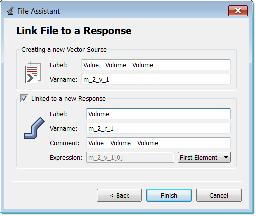
| g. | Click Finish. The Volume output response is added to the work area. |
| 2. | Create the Stress43 output response, which represents the von Mises Stress of Element 43. |
| a. | From the Directory, drag-and-drop the plate1.h3d file, located in the approaches/nom_1/run__00001/m_1 directory, into the work area. This file contains the analysis results, including stresses. |
| b. | In the File Assistant dialog, set the Reading technology to Altair® HyperWorks® and click Next. |
| c. | Select Single item in a time series, then click Next. |
| d. | Define the following options, then click Next. |
| • | Set Subcase to Subcase 1(Load). |
| • | Set Type to Element Stresses (2D & 3D) (2D). |
| • | Set Component to vonMises (Mid). |
| e. | Label the output response Stress43. |
| f. | Set Expression to First Element. |
| g. | Click Finish. The Stress43 output response is added to the work area. |
| 3. | Create the Frequency1 output response, which represents frequency results. |
| a. | From the Directory, drag-and-drop the plate2.out file, located in the approaches/nom_1/run__00001/m_2 directory, into the work area. This file contains the analysis results, including stresses. |
| b. | In the File Assistant dialog, click Next. |
| c. | Select Single item in a time series, then click Next. |
| d. | Define the following options, then click Next. |
| e. | Label the output response Frequency1. |
| f. | Set Expression to First Element. |
| g. | Click Finish. The Frequency1 output response is added to the work area. |
| 4. | Click Evaluate Expressions to extract the output response values. |
|
| 1. | In the Explorer, right-click and select Add Approach from the context menu. |
| 2. | In the HyperStudy - Add dialog, select Optimization and click OK. |
| 3. | Go to the Select Input Variables step. |
| 4. | Review the input variable's lower and upper bound ranges. |
| 5. | Go to the Select Output Responses step. |
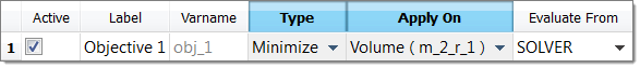
| 7. | In the HyperStudy - Add dialog, add one objective. |
| b. | Set Apply On to Volume (m_2_r_1). |
| 9. | Click the Constraint tab. |
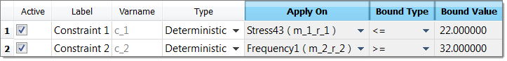
| 11. | In the HyperStudy - Add dialog, add two constraints. |
| 12. | Define Constraint 1 and Constraint 2 by selecting the options indicated in the image below from the Apply On, Bound Type, and Bound Value columns. |
| 14. | Go to the Specifications step. |
| 15. | In the work area, set the Mode to Adaptive Response Surface Method (ARSM). |
| Note: | Only the methods that are valid for the problem formulation are enabled. |
| 17. | Go to the Evaluate step. |
| 19. | Click the Iteration Plot tab to plot the progress of the Optimization iteration. |
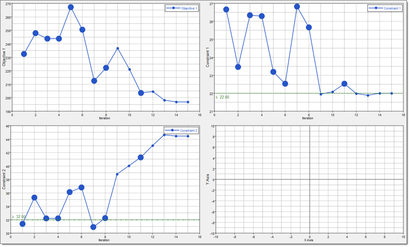
Using the Channel selector, select Objective 1, Constraint 1, and Constraint 2. Above the Channel selector, activate multiplot and enable the Bounds setting.
Over the course of the optimization, the objective is minimized and at the conclusion, the constraints are satisfied. In the plots, the large markers indicate a design which has at least one violated constraint and a small marker indicates a feasible design. At the optimal design, the only active constraint is Constraint 1. In contrast, constraint 2 is not active at the optimum; this indicates Constraint 2 does not have an influence on the result.
|
See Also:
HyperStudy Tutorials


