This tutorial demonstrates how to perform a multi-disciplinary design optimization study. The disciplines used in this tutorial are structural performance and cost. Structural performance is simulated using OptiStruct and Cost is simulated using HyperMath. Optimization parameters for both the simulations are identified in template files corresponding to each input deck (tail_structure.fem and tail_cost.hml).The sample base input templates used in this tutorial can be found in <hst.zip>/HS-4215/ and copied to your working directory. The tutorial directory includes the following files:
tail_structure_radioss.tpl
|
Base input parameterized file model 1.
|
tail_cost_hypermath.tpl
|
Base input parameterized file model 2.
|
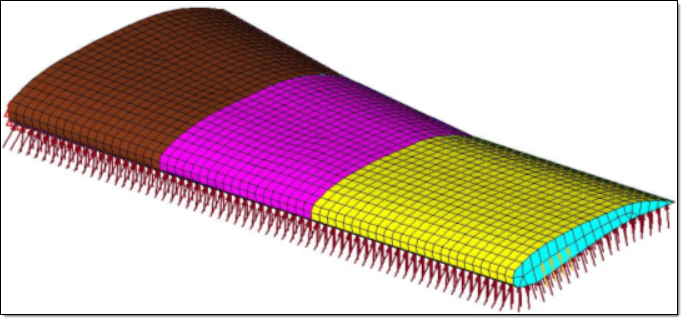
Horizontal tail plane model
It is assumed that the tail is cantilevered about its inboard section. Three loading scenarios are considered; one where the tail experiences pressure loads of 0.25 psi on the bottom skin, a second where the tail experiences a tip load of 400 lbs, and a third where the tail experiences both the pressure load and tip load simultaneously. The applied loading is represented in the following figure.
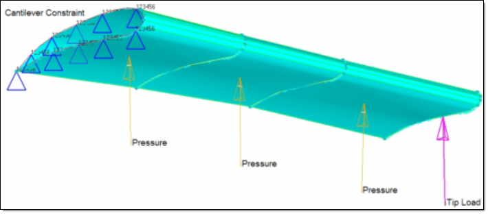
Loading experienced by horizontal tail plane
Problem Formulation for this study is as follows:
Input variables:
| • | glass fabric thickness at inboards; initial value = 0.1; lower bound = 0.01, upper bound = 2.0 |
| • | glass fabric thickness at midspan; initial value = 0.1; lower bound = 0.01, upper bound = 2.0 |
| • | glass fabric thickness at outboards; initial value = 0.1; lower bound = 0.01, upper bound = 2.0 |
| • | core thickness at inboards; initial value = 0.1; lower bound = 0.01, upper bound = 2.0 |
| • | core fabric thickness at midspan; initial value = 0.1; lower bound = 0.01, upper bound = 2.0 |
| • | core fabric thickness at outboards; initial value = 0.1; lower bound = 0.01, upper bound = 2.0 |
| • | aluminum rib thickness; initial value = 0.1; lower bound = 0.01, upper bound = 2.0 |
| Note: | Both models have seven input variables; however values of the input variables need to be consistent between the two models. In order to obtain this, we will be linking the two sets of input variables to each other. |
|
Objective:
To minimize the cost.
Design constraints:
Maximum displacement must be less than its baseline value of 31.
| 2. | To start a new study, click File > New from the menu bar, or click  on the toolbar. on the toolbar. |
| 3. | In the HyperStudy – Add dialog, enter a study name, select a location for the study, and click OK. |
| 4. | Go to the Define models step. |
| 5. | Add a Parameterized File model. |
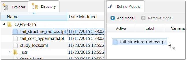
| a. | From the Directory, drag-and-drop the tail_structure_radioss.tpl file into the work area. |
| b. | In the Solver input file column, enter tail.fem. This is the name of the solver input file HyperStudy writes during any evaluation. |
| c. | In the Solver execution script column, select OptiStruct (os). |
| 6. | Add a Parameterized File model. |
| a. | From the Directory, drag-and-drop the tail_cost_hypermath.tpl file into the work area. |
| b. | In the Solver input file column, enter tail.hml. This is the name of the solver input file HyperStudy writes during any evaluation. |
| c. | In the Solver execution script column, select HyperMath (hmath). |
| d. | In the Solver input arguments column, enter -f before $file. |

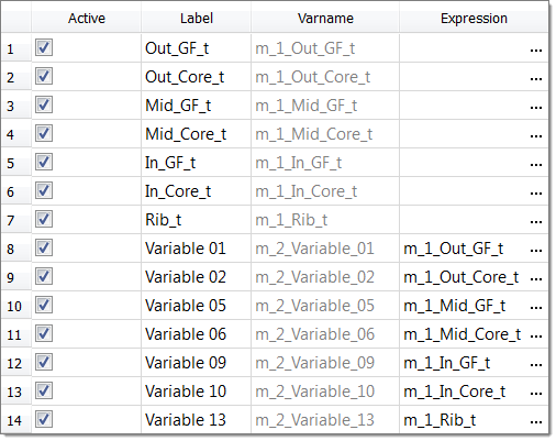
| 7. | Click Import Variables. Fourteen input variables are imported from the tail_structure_radioss.tpl and tail_cost_hypermath.tpl resource files. |
| 8. | Go to the Define Input Variables step. |
| 9. | Review the input variable's lower and upper bound ranges. |
| 10. | Click the Link Variables tab. |
| 11. | In the Varname column, copy all of the independent variables (all variables from Model_1). |
| 12. | In the Expression column of all of the dependent input variables (all variables from Model_2), paste the independent variables. |
| 13. | Go to the Specifications step. |
|
| 1. | In the work area, set the Mode to Nominal Run. |
| 3. | Go to the Evaluate step. |
| 4. | Click Evaluate Tasks. An approaches/nom_1/ directory is created inside the study directory. The approaches/nom_1/run__00001/m_1 and approaches/nom_1/run__00001/m_2 sub-directories contain the tail.h3d (for maximum displacement) and cost.res (for cost) files, which are the result of the nominal run, and will be used in the optimization. |
| 5. | Go to the Define Output Responses step. |
|
In this step you will create two output responses: MaxDisp and Cost.
| 1. | Create the MaxDisp output response. |
| a. | From the Directory, drag-and-drop the tail.h3d file, located in the approaches/nom_1/run__00001/m_1 directory, into the work area. |
| b. | In the File Assistant dialog, set the Reading technology to Altair® HyperWorks® and click Next. |
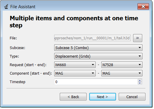
| c. | Select Multiple items at one time step (resvector), then click Next. |
| d. | Define the following options, then click Next. |
| • | Set Subcase to Subcase 5 (Combo). |
| • | Set Type to Displacement (Grids). |
| • | Set Request (start - end) to N4660 - N7528. |
| • | Set Component (start - end) to Mag - Mag. |
| e. | Label the output response MaxDisp. |
| f. | Set Expression to Maximum. |
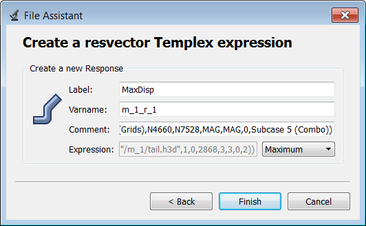
| g. | Click Finish. The MaxDisp output response is added to the work area. |
| 2. | Create the Cost output response. |
| a. | From the Directory, drag-and-drop the hmat.res file, located in the approaches/nom_1/run__00001/m_2 directory, into the work area. This file contains the analysis results, including stresses. |
| b. | In the File Assistant dialog, set the Reading technology to Altair® HyperWorks® and click Next. |
| c. | Select Single item in a time series, then click Next. |
| d. | Define the following options, then click Next. |
| • | Set Component to Column 1. |
| e. | Label the output response Cost. |
| f. | Set Expression to First Element. |
| g. | Click Finish. The Cost output response is added to the work area. |
| 3. | Click Evaluate Expressions to extract the output response values. |

|
| 1. | In the Explorer, right-click and select Add Approach from the context menu. |
| 2. | In the HyperStudy - Add dialog, select Optimization and click OK. |
| 3. | Go to the Select Input Variables step. |
| 4. | Review the input variable's lower and upper bound ranges. |
| 5. | Go to the Select Output Responses step. |
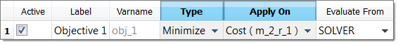
| 7. | In the HyperStudy - Add dialog, add one objective. |
| b. | Set Apply On to Cost (r_2). |
| 9. | Click the Constraint tab. |
| 11. | In the HyperStudy - Add dialog, add one constraint. |
| 12. | Define the constraint. |
| a. | Set Apply On to MaxDisp ( r_1). |
| b. | Set Bound Type to <= (less than or equal to). |
| c. | For Bound Value, enter 31.0. |

| 14. | Go to the Specifications step. |
| 15. | In the work area, set the Mode to Adaptive Response Surface Method (ARSM). |
| Note: | Only the methods that are valid for the problem formulation are enabled. |
| 17. | Go to the Evaluate step. |
|
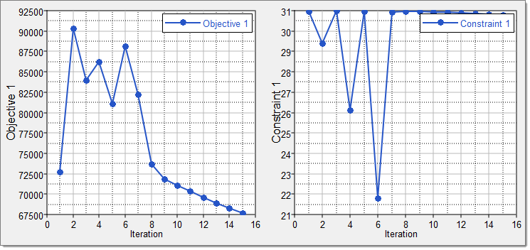
Click the Iteration Plot tab to plot the progress of the Optimization iteration..
Using the Channel selector, select Objective_1 and Constraint_1. The evolution of the objective function and constraint vs. iterations is 2D plotted. You can see that the cost of the horizontal tail plane is reduced from 72715 to 67700 (7% reduction), while keeping the structural performance the same.
|
See Also:
HyperStudy Tutorials


