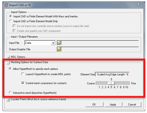
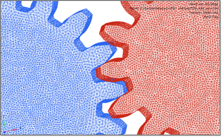
New meshing options are now available when importing CAD geometry. These enable you to control the mesh density in a very intuitive way.

Accurate contact force generation requires uniform meshes. New algorithms, more suited for uniform mesh generation are now used.  This new meshing option is only enabled for input geometries and not for FE models.

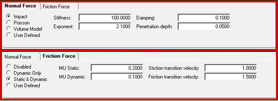
The Properties tab in the Contact panel has been reorganized to have sub-tabs for normal force and friction force.

Reasonable contact and friction parameters are provided as defaults. You do not have to change these unless your contacts have special properties.

Parameters are checked for validity as they are entered and the user is alerted to invalid values before the model is run.

Output Requests to measure contact forces are automatically created.

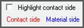
All contact meshes examined and invalid or “dirty” geometry is clearly identified during modeling.  Contact surfaces for all meshes can be visualized using “Highlight contact side” option in the Connectivity tab.

Surface normals can be inverted with just one operation. This is especially useful when contact is happening inside a selected closed geometry.

Red indicates outward normals and blue indicates the inward normals.

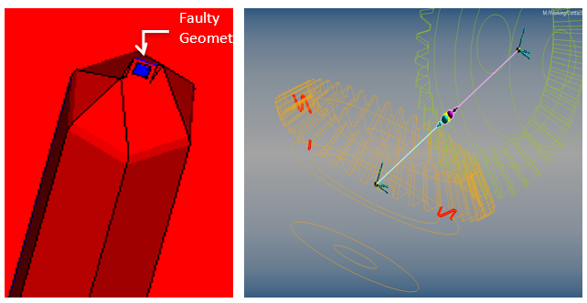
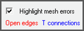
The normals for a mesh are automatically corrected when inconsistencies are detected. This is especially useful when tria-meshes are imported from STL files or Wavefront OBJ files.

Open edges and T connections, if any, can be highlighted as shown in the figure on the top right. If the mesh is clean (i.e. it forms a closed volume), the panel indicates “No mesh errors” else the “Highlight mesh errors” option becomes available.

MotionView now includes a new mesh manipulation tool that allows you to clean previously unusable meshes for contact solution. The capability is accessed from the Import CAD or FE utility.

Import CAD or FE utility now provides additional cleaning options that enable you to fill holes, thicken surfaces, eliminate T-junctions and shrink-wrap unusable meshes. All of this is done with a minimum of user input.

A new Volume Model for normal force calculations is now supported. User defined contact models for both normal and friction forces are also supported.

In addition, user-defined normal and friction force definitions are supported.

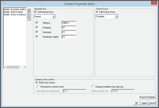
This macro tool has been updated to take into account the new contact properties available in the solver and makes setting properties across multiple contacts quick and intuitive.

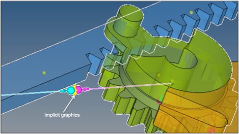
A new “implicit graphics” contact icon is now visible. You can visually see the geometries that have contact connections.

Associated graphics are highlighted when contact entity is selected.

Advanced options are available to detect the precise event when contact occurs. An option is also available to change the maximum step size subsequent to contact detection. This option introduces a Sensor entity with a zero crossing attribute into the MotionSolve XML file. This Sensor will control integration step size so that the onset of contact is accurately detected.

Refer to Rigid to Rigid Contact section in MotionView User Guide to learn more about modeling contacts.

A new collision engine that vastly improves the robustness of mesh-mesh contact has been implemented.

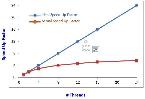
There are two main reasons for fast contact simulations:

Parallel solution for all contacts

The contact kinematics between each pair of geometries is calculated in parallel in different threads. This means whenever there are multiple contacts in your model you can improve simulation time by using multiple cores in a machine. All contact pairs will be dynamically distributed onto the available cores.

The graph below shows how contact simulations speed up as a function of the number of threads used to solve for contact.

Specialized contact algorithms for simpler shapes

A much faster, specialized sphere-to-mesh contact algorithm is now available.

A much faster, specialized sphere-to-sphere contact algorithm is now available.

Both of these are automatically invoked when needed.

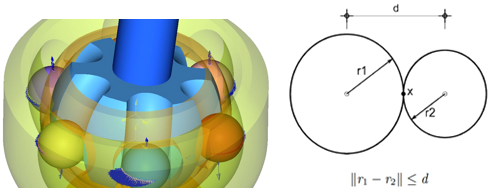
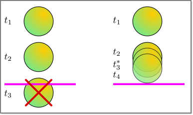
A zero crossing sensor that monitors the distance between contacting geometries is now available. The zero crossing sensor controls integrator step-size to precisely capture the contact event.

Note: This sensor is only meaningful for impulsive contacts. If a contact is persistent, then a zero crossing sensor is not needed.

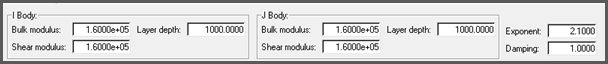
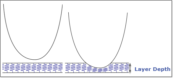
A new “Volume” force model that relies on understandable physical parameters such as bulk modulus and shear modulus is now available.

The normal force is based on an Elastic foundation model. The rigid bodies in contact are assumed to be covered by thin elastic layers. If the tangential shear stress in the layer is ignored, a direct relationship can be found between the normal pressure and normal displacement. This relationship can be used to generate the force between two contacting layers. This model is well known in the literature for contacts.

An option to output the system state at the maximum penetration depth in-between two regular output steps is now available. When you run a simulation from MotionView, this is done automatically. You can filter out these “extra” outputs in HyperView.

The CONTACT () function has been enhanced to provide many more details about the contact such as maximum penetration depth, number of contact patches, total number of contacts, area of contact, etc.

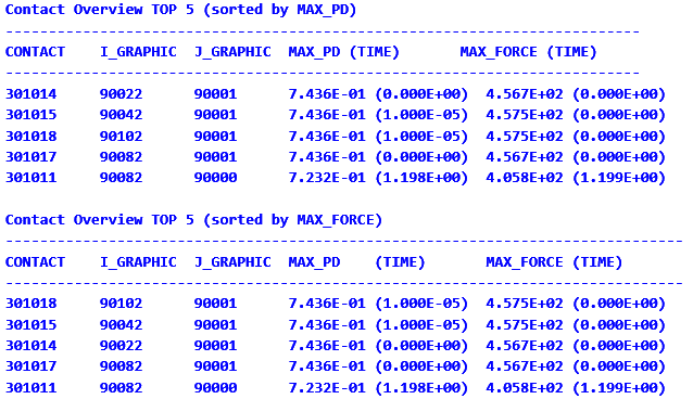
Contact metrics tables are now printed in the MotionSolve log file. You can examine the metrics table to determine what the maximum penetration(s) and normal force(s) is/are in your model and when it occurred. Two tables are printed – one ordered by maximum penetration depth and another ordered by maximum contact force:

A contact report containing this table is also available in MotionView.

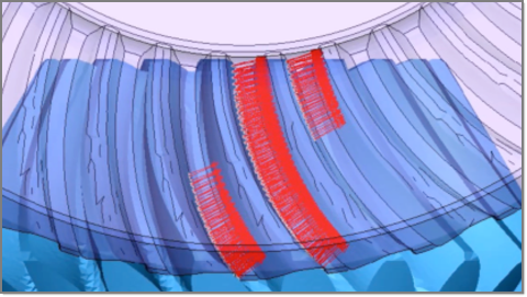
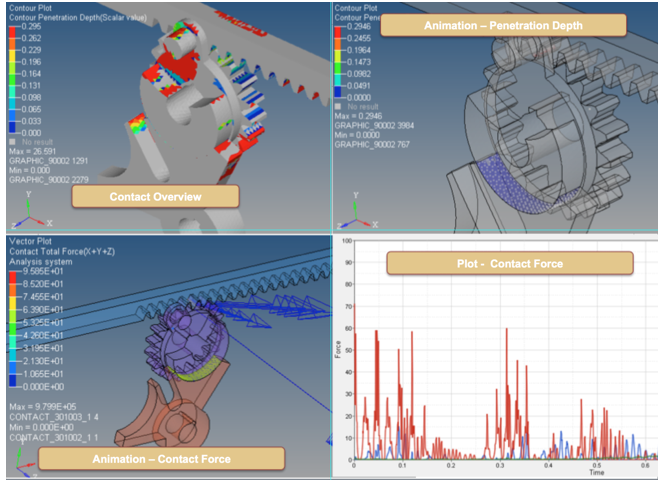
New vector plots are now available for visualizing normal force, friction force, penetration depth, and penetration velocity.

The coefficient of friction in the contact patches can now be visualized as a contour plot.

Contact forces by region can now be visualized.

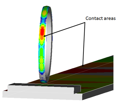
A new contact summary frame is now available in HyperView. This summary frame will show you where contact has occurred during a simulation with a contour of the maximum penetration depth for all contact occurrences through the entire length of the simulation.

MotionView now has capability to generate a Contact Report automatically to simplify the post processing of contacts.

For every model that involves contacts, the auto-generated report contains the necessary plots and animations that enable you to easily understand contact behavior in your model.

New options have been added to the contact function. This enables you to create requests containing contact details that can be easily plotted.