Title
Snap Roof - Explicit
|
|
Number
2.1
|
Brief Description
An imposed velocity is applied onto a shallow cylindrical roof at its midpoint. The analysis uses an explicit approach.
|
Keywords
| • | Elasticity and quasi-static analysis |
| • | Stability, snap-through problem, and limit load |
|
RADIOSS Options
| • | Boundary conditions (/BCS) |
|
Compared to / Validation Method
|
Input File
Explicit solver: <install_directory>/demos/hwsolvers/radioss/02_Snap-through/Explicit_solver/SNAP_EXP*
|
Technical / Theoretical Level
Beginner
|
Overview
Aim of the Problem
The purpose of this example is to study a snap-thru problem with a single instability. Thus, a structure that will bend when under a load is used. The results are compared to the references contained in: Finite Element Instability Analysis of Free Formed Shells. Report 77−2, 1977, Norwegian Institute Of Technology, Trondheim, HORRIGMOE G.
This static analysis is performed with an explicit approach.
Physical Problem Description
A shallow cylindrical roof, pinned along its straight edges upon which an imposed velocity is applied at its mid-point.
Units: mm, ms, g, N, MPa
Geometrical data are provided in Fig 1, with the following dimensions:
| • | Shell thickness: t = 12.7 mm |
| • |  = 0.1 rad = 0.1 rad |
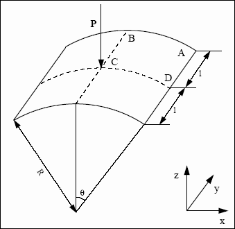
Fig 1: Geometrical data of the problem
The material used follows a linear elastic law and has the following characteristics:
| • | Initial density: 7.85x10⁻³ g/mm3 |
| • | Young modulus: 3102.75 MPa |
Analysis, Assumptions and Modeling Description
Modeling Methodology
The structure is considered perfect, having no defects. To take account of the symmetries, only a quarter of the shell is modeled (surface ABCD).
A regular mesh with a total of 72 3-node shells (Fig 2)
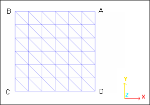
Fig 2: T3 mesh
The shells have the following properties:
| • | BT Elasto-plastic Hourglass formulation (Ishell = 3). |
RADIOSS Options Used
Node time histories do not indicate the pressure output. In order to obtain such output at point C, a rigid body must be created at this point. Point C has a constant imposed velocity of -0.01 ms-1 in the Z direction. Its displacement is linked proportionally to time.
Boundary conditions are:
| • | Edge BC is fixed in an X translation, and in Y and Z rotations (symmetry conditions). |
| • | Edge CD is fixed in a Y translation, and in X and Z rotations (Idem). |
| • | Edge DA is fixed in X, Y, Z translations, and in X and Z rotations. |
| • | Point C is fixed in X, Y translations, and in X, Y, Z rotations. |
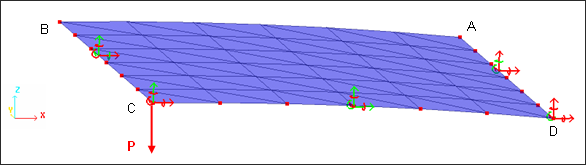
Fig 3: Boundary conditions
Simulation Results and Conclusions
Curves and Animations
Only a quarter of the total load is applied due to the symmetry. Therefore, force Fz of the rigid body, as indicated in the Time History, must be multiplied by 4 in order to obtain force, P.
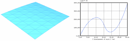
Figure 4 represents a characteristic load displacement curve for a snap-through. This diagram plots the reaction at point C of the shell as a function of its vertical displacement.
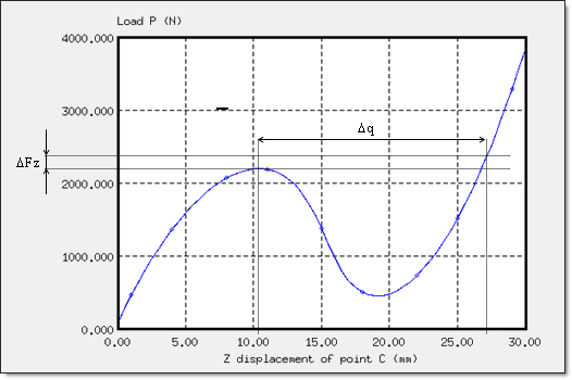
Fig 4: Load P versus displacement of point C: snap-thru instability.
The displacement of point C is indicated in its absolute value. The curve illustrates the characteristic behavior of the instability of a snap-thru. Beyond the limit load, an infinite increase in load  Fz will cause a considerable increase in displacement q due to the collapsing of the shell.
The first extreme defines the limit load =2208.5 N (displacement of point C = 10.5 mm).
The increase in the curve slope after the snap-thru, shows that the deformed configuration becomes more rigid.
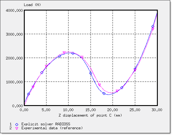
Fig 5: Comparison between a reference curve and a curve obtained using RADIOSS
The difference between the two curves is approximately 10% for reduced displacements (up to 5 mm) and slightly more (15%) for the higher nonlinear part of the curve (between 5 and 20 mm). For displacements exceeding 20 mm, the curves are shown much closer together.
The accuracy of the RADIOSS results in comparison to those obtained from the reference is ideal for this explicit approach.
Deformed Mesh (profile view) – Displacement Norm
|
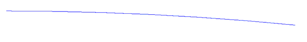
Initial configuration
|

Start of snap-thru
|

Large motion phase
|

Stable configuration
|
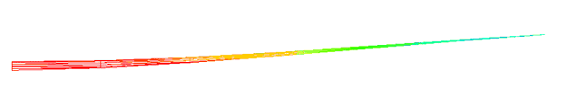
Loading with a new structural rigidity
|


