Title
Snap Roof - Implicit
|
|
Number
2.2
|
Brief Description
A shallow cylindrical roof upon which an imposed velocity is applied at its mid-point. Analysis uses an implicit approach.
|
Keywords
| • | Implicit solver, time step control by arc-length method |
| • | Static nonlinear analysis |
| • | Stability, snap-thru, and limit load |
|
RADIOSS Options
| • | Boundary conditions (/BCS) |
| • | Implicit options (/IMPL) |
|
Compared to / Validation Method
|
Input File
Implicit solver: <install_directory>/demos/hwsolvers/radioss/02_Snap-thru/Implicit_solver/SNAP_IMP*
|
Technical / Theoretical Level
Advanced
|
Overview
Aim of the Problem
The purpose of this example is to study a snap-thru problem with a single instability. Thus, a structure that will bend when under a load will be used. The results are compared to a reference solution [1]. This analysis is performed using an implicit approach. An implicit strategy using an arc-length method is illustrated.
Physical Problem Description
A shallow cylindrical roof, pinned along its straight edges, upon which an imposed velocity is applied at its mid-point.
Units: mm, ms, g, N, MPa
Geometrical data are indicated in Fig 6, with the following dimensions:
| • | Shell thickness: t = 12.7 mm |
| • |  = 0.1 rad = 0.1 rad |
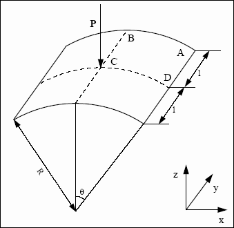
Fig 6: Geometrical data of the problem
The material used follows a linear elastic law and has the following characteristics:
| • | Initial density: 7.85x10⁻³ g/mm3 |
| • | Young modulus: 3102.75 MPa |
Analysis, Assumptions and Modeling Description
Modeling Methodology
The modeling problem described in the explicit study remains unchanged.
The implicit computation requires specific implicit parameters that must be defined in the Engine file *_001.rad using the options beginning with /IMPL.
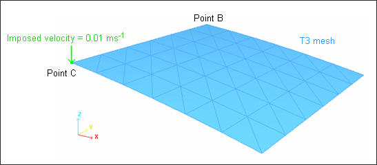
Fig 7: Description of the problem (one quarter of the shell is modeled)
The imposed velocity is considered using the implicit method. Thus, the constant input curve is converted into an imposed displacement according to the computation time.
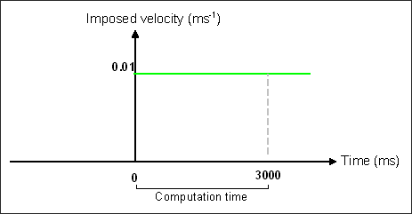
Fig 8: Imposed velocity curve
RADIOSS Options Used
The limit point causes major non-linearities. Therefore, a static nonlinear analysis is performed using the arc-length displacement strategy. The time step is determined by a displacement norm control. In order to exceed the limit point characterized by a null tangent on the load displacement curve and to describe the increasing and decreasing parts of the nonlinear path, a small time step is required, which is ensured by setting a maximum value.
The nonlinear implicit parameters used are:
| Implicit type: | Static nonlinear |
| Nonlinear solver: | Modified Newton |
Tolerance: 2x10⁻⁴
| Update of stiffness matrix: | 3 iterations maximum |
| Time step control method: | Arc-length |
| Minimum time step: | 0.5 ms |
| Desired convergence iteration number: | 6 |
| Maximum convergence iteration number: | 20 |
| Decreasing time step factor: | 0.8 |
| Maximum increasing time step scale factor: | 1.05 |
| Arc-length: | Automatic computation |
A solver method is required to resolve Ax=b in each iteration of a nonlinear cycle. It is defined in /IMPL/SOLVER. The linear implicit options used are:
| Linear solver: | Direct solver MUMPS |
| Precondition methods: | Factored approximate Inverse |
| Maximum iterations number: | System dimension (NDOF) |
| Stop criteria: | Relative residual in force |
| Tolerance for stop criteria: | Machine precision |
The input implicit options set in *_001.rad are:
/IMPL/PRINT/NONL/-1
|
Printout frequency for nonlinear iteration
|
/IMPL/SOLVER/2
5 0 0 0.0
|
Solver method (solve Ax=b)
|
/IMPL/NONLIN
3 1 0.20e-3
|
Static nonlinear computation
|
/IMPL/DTINI
10
|
Initial time step determines the initial loading increment
|
/IMPL/DT/STOP
0.5 10
|
Min Max values for time step
|
/IMPL/DT/2
6.0 20 0.8 1.05
|
Time step control method 2 - Arc-length+Line-search will be used
with this method to accelerate and control convergence
|
Refer to RADIOSS Starter Input for more details about implicit options.
Simulation Results and Conclusions
Curves and Animations
Only a quarter of the total load is applied due to the symmetry. Thus, force Fz of the rigid body as indicated in the Time History must be multiplied by 4 in order to obtain force, P.
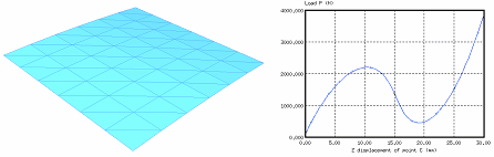
Figure 9 represents the characteristic load displacement curve for a snap-thru. This diagram plots the reaction at point C of the shell as the function of its vertical displacement. The implicit results are compared with the experimental data.
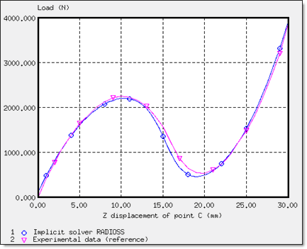
Fig 9: Load P versus displacement of point C.
For a time step equal to or less than 10 ms (maximum value set in the implicit /IMPL/DT/STOP option), agreement with RADIOSS is achieved, with good results obtained using the reference. Accuracy is improved by decreasing the maximum time step, even though the CPU time is increased.
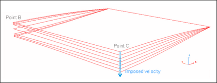
Fig 10: Deformed configurations during the snap-thru.
Comparison between Implicit and Explicit Results
The load displacement curves achieved through implicit computations (time step limit set to 10 ms) and explicit computations are very close. A maximum time step of 100 ms does not allow the nonlinear path of the load displacement curve to be described accurately. However, the final static solution is correct.
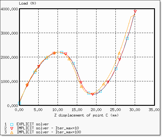
Fig 11: Load displacement curve obtained by implicit and explicit solvers.
Comparison of the computation time between the explicit and implicit (maximum time step set to 10 ms) approaches is shown in the table below:
|
Implicit solver
|
Explicit solver
|
Normalized CPU
|
1
|
2.45
|
Cycles (normalized)
|
1
|
237
|
In comparison with the implicit computation, which uses a maximum time step of 10 ms, the saved CPU time using a maximum time step fixed at 100 ms, approximately corresponds to factor 4.
Reference
[1] Finite Element Instability Analysis of Free Formed Shells. Report 77−2, 1977, Norwegian Institute Of Technology, Trondheim, HORRIGMOE G.


