Summary
Polynomial EOS is often used by RADIOSS to compute hydrodynamic pressure. It is cubic in compression and linear in expansion.
where,
 (1) and
  (2)
(2)
Material law 6 (/MAT/HYDRO) uses this equation to compute hydrostatic pressure. It is possible to consider absolute values or relative variation (Table 1). This example shows how to build material control cards for each of the following cases:
Case
|
Mathematical model
|
Pressure
|
Energy
|
1
|

|
absolute
|
absolute
|
2
|

|
relative
|
absolute
|
3
|

|
relative
|
relative
|
4
|

|
absolute
|
relative
|
Table 1: Modeling formulation for perfect gas with /MAT/HYDRO
A simple test of compression/expansion is made to compare these formulation outputs with theoretical results.
Title
Perfect Gas Modeling with
Polynomial EOS
|
|
Number
43.1
|
Brief Description
Polynomial EOS is used to model perfect gas. Pressure or energy can be absolute values or relative. Material law 6 (/MAT/HYDRO) is used to build material cards for each of these cases.
|
Keywords
| • | Absolute/Relative formulations |
|
RADIOSS Options
| • | Hydrodynamic fluid material (/MAT/LAW6 (HYDRO)) |
|
Compare to / Validation method
Input File
Model 1: <install_directory>/demos/hwsolvers/radioss/43_perfect_gas_polynomial_eos/01-Pabsolute_Eabsolute/*
Model 2: <install_directory>/demos/hwsolvers/radioss/43_perfect_gas_polynomial_eos/02-Prelative_Eabsolute/*
Model 3: <install_directory>/demos/hwsolvers/radioss/43_perfect_gas_polynomial_eos/03-Prelative_Erelative/*
Model 4: <install_directory>/demos/hwsolvers/radioss/43_perfect_gas_polynomial_eos/04-Pabsolute_Erelative/*
|
Technical / Theoretical Level
Beginner
|
Overview
Aim of the Problem
The purpose of this example is to plot numerical pressure, internal energy, and sound speed for a perfect gas material law. Comparison to theoretical results is made.
Physical Problem Description
This test consists with an elementary volume of perfect gas undergoing spherical expansion and compression.
Initial conditions are listed below:
P0 = 1e5 Pa
V0 = 1000 m3
 0 = 1.204 kg/m3
 0 = 0
0 = 0
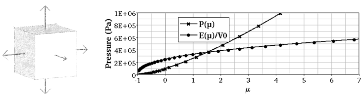
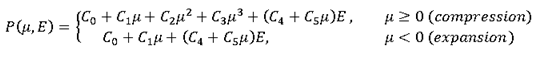
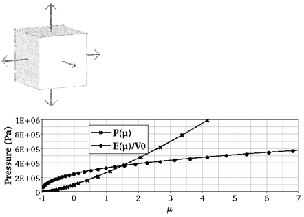
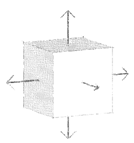
The fluid will be assumed to be a perfect gas. Volume is changed in the three directions to consider a pure compression (-1 < < 0) followed by an expansion of matter (0 < ). See Figure 1.
This test will be modeled with a single ALE element (8 node brick) and polynomial EOS.
Evolutions of pressure, internal energy and sound speed will be compared between numerical output and theoretical results.
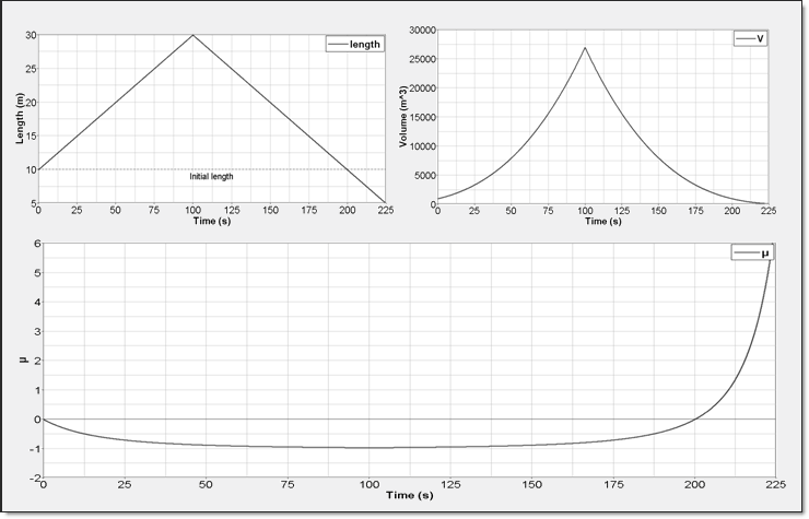
Fig 1: Elementary volume change. Length is modified with /IMPDISP card; its influences on V and are plotted.
Analysis, Assumptions and Modeling Description
RADIOSS Options Used
Nodes on each of the faces are moved with imposed displacement (/IMPDISP).
Boundary nodes are defined as Lagrangian with the /ALE/BCS card.
Element pressure, density and internal energy density are saved in the Time History file.
Polynomial EOS
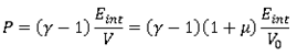
Polynomial EOS is used in material law 6 (/MAT/HYDRO) to compute hydrodynamic pressure. It is cubic in compression and linear in expansion.
Where, P is the hydrodynamic pressure.
(1)
and
(2)
 are called hydrodynamic coefficients and they are input flags. Hypothesis on the material behavior allows determining of these coefficients:
| • | General case corresponds to Mie-Guneisen EOS (see Appendix C of the Theory Manual) |
This example is focused only on Perfect Gas modeling.
Theoretical Results
The purpose of this section is to plot pressure, internal energy, and sound speed in function of the single parameter V or .
Perfect gas pressure is given by:
 (3)
(3)
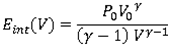
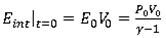
Then,
RADIOSS assumes the hypothesis of an isentropic process to compute the change in internal energy:
dEint = -PdV
This theory gives the following differential equation:

This has the form  and the general solution is:

Pressure is also polytropic:
 | (4) |
Here,  is the material constant (ratio of heat capacity). For diatomic gas =1.4. Air is made mainly of diatomic gas, so set gamma to 1.4 for air.
Equations (3) and (4) lead to the immediate result:
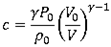
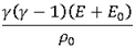
Perfect gas sound speed is:
 | (5) |
Equation (4) gives its expression in term of volume:
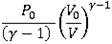
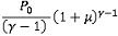
The theoretical results are listed in the table below. Pressure, internal energy, and sound speed are expressed both in function of V and .
Pressure (Pa)
|
Internal Energy Density (J)
|
Sound Speed (m/s)
|
PREF(V)
|
PREF()
|
eREF(V)
|
eREF()
|
cREF(V)
|
cREF()
|

|

|
|
|

|

|
Corresponding plots are shown below:
Fig 2: Perfect Gas Pressure
Fig 3: Perfect Gas Internal Energy
Fig 4: Perfect Gas Sound Speed
Modeling Methodology
A single ALE brick element is used. Material is confined inside the element by defining brick nodes as Lagrangian. For each face, displacement is imposed on the four nodes along the normal.
Material law 6 (/MAT/HYDRO) is used and describes the hydrodynamic viscous fluid material.
(1)
|
(2)
|
(3)
|
(4)
|
(5)
|
(6)
|
(7)
|
(8)
|
(9)
|
(10)
|
/MAT/LAW6/mat_ID/unit_ID or /MAT/HYDRO/mat_ID/unit_ID
|
mat_title
|

|
|
|
|
|
|
|
|

|
|
|
|
|
|
|
|
|
C0
|
C1
|
C2
|
C3
|
|
|
Pmin
|
Psh
|
|
|
|
|
|
|
C4
|
C5
|
E0
|
|
|
|
|
Pressure Shift
Material law 6 introduces flag Psh which allows shifting computed pressure in the polynomial equation of state:
RADIOSS Engine shifts C0 flag and computed pressure P( ,E) with an offset of -Psh.
Minimum Pressure
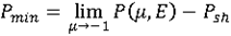
The theoretical value is Pmin = 0 Pa (absolute pressure) with a default value of -1030, to accept a negative value in relative pressure formulation.
This flag has to be manually offset with -Psh.
Simulation Results and Conclusions
Material Control Cards
Material is supposed to be a perfect gas. The following cases have been investigated:
| • | Case 1: Both Pressure and Energy are absolute values:  |
| • | Case 2: Pressure is relative and Energy is absolute:  |
| • | Case 3: Both Pressure and Energy are relative:  |
| • | Case 4: Pressure is absolute and Energy is relative:  |
Equation of state can be written:
with
Expanding this expression and identifying the polynomial coefficients leads to:
where,
(1)
|
(2)
|
(3)
|
(4)
|
(5)
|
(6)
|
(7)
|
(8)
|
(9)
|
(10)
|
/MAT/LAW6/mat_ID/unit_ID or /MAT/HYDRO/mat_ID/unit_ID
|
AbsolutePRESSURE_AbsoluteENERGY
|

|
|
|
|
|
|
|
|
|
|
|
|
|
|
|
|
|
0
|
0
|
0
|
0
|
|
|
0
|
0
|
|
|
|
|
|
|
C4 = - 1
|
C5 = - 1
|

|
|
|
|
|
Time History
|
Measure
|
Initial Value
|
Unit
|
/TH/BRICK (P)
|
P
|
P0
|
Pressure
|
/TH (IE)
|
Eint (= E x V0)
|
E0V0
|
Energy
|
/TH/BRICK (IE)
|
Eint / V
|
E0
|
Pressure
|
| 4. | Comparison with Theoretical Result |
Numerical result for perfect gas pressure is given by time history. Element time history (RADIOSS /TH/BRICK) allows displaying it. This result is compared to a theoretical one. Curves are superimposed.
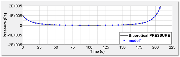
Fig 5: Numerical pressure, model 1:
Internal energy can be obtained through two different ways. The first one is internal energy density (Eint / V) recorded by element time history (RADIOSS /TH/BRICK). The second one is the internal energy from the global time history  because the model is composed of a single element. because the model is composed of a single element.
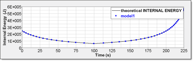
Fig 6: Numerical internal energy, model 1: 
|
Equation of state for a perfect gas is:
Calculating Pressure from a reference one provides relative pressure:
Expanding this expression and identifying with polynomial coefficients leads to:
 P(,E) = P(,E) = Psh = -Psh + (C4 + C5)E P(,E) = P(,E) = Psh = -Psh + (C4 + C5)E
where,
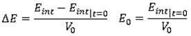
Then, the minimum pressure must be set to a non-zero value Pmin = -P0.
(1)
|
(2)
|
(3)
|
(4)
|
(5)
|
(6)
|
(7)
|
(8)
|
(9)
|
(10)
|
/MAT/LAW6/mat_ID/unit_ID or /MAT/HYDRO/mat_ID/unit_ID
|
RelativePRESSURE_AbsoluteENERGY
|

|
|
|
|
|
|
|
|
|
|
|
|
|
|
|
|
|
0
|
0
|
0
|
0
|
|
|
-P0
|
P0
|
|
|
|
|
|
|
C4 = - 1
|
C5 = - 1
|
|
|
|
|
|
Time History
|
Measure
|
Initial Value
|
Unit
|
/TH/BRICK (P)
|
P
|
0
|
Pressure
|
/TH (IE)
|
Eint (= E x V0)
|
E0V0
|
Energy
|
/TH/BRICK (IE)
|
Eint / V
|
E0
|
Pressure
|
| 5. | Comparison with Theoretical Result |
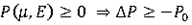
Element time history (/TH/BRICK) is the pressure relative to Psh. The resulting curve is then shifted with Psh value and starts from 0.
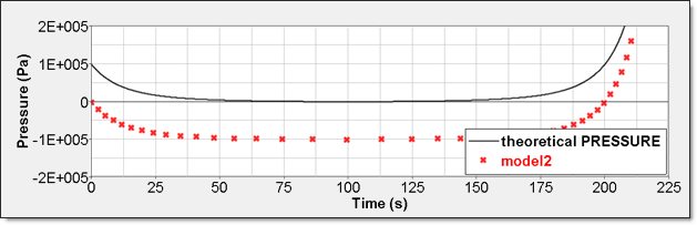
Fig 7: Numerical pressure, model 2:
Internal energy can be obtained through two different ways. The first one is internal energy density (Eint / V) recorded by element time history (/TH/BRICK). The second one is the internal energy from the global time history because the model is composed of a single element.
Fig 8: Numerical internal energy, model 2: 
|
Equation of state for a perfect gas is:
Initial internal energy can be introduced:
Calculating pressure from a reference one provides:
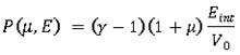
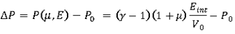
P(,E) - P0 = P = ( - 1)(1 + )(E + E0) - P0
Where,
Expanding this expression and identifying with polynomial coefficients leads to:
P(,E) = P( ,E) - Psh = C0 - Psh + C1 + (C4 + C5)E
where,
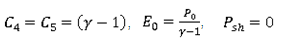
C0 = C1 = E0( - 1)
C4 = C5 = - 1
E0 = 0
Psh = P0
The minimum pressure must be set to a non-zero value Pmin = -P0
(1)
|
(2)
|
(3)
|
(4)
|
(5)
|
(6)
|
(7)
|
(8)
|
(9)
|
(10)
|
/MAT/LAW6/mat_ID/unit_ID or /MAT/HYDRO/mat_ID/unit_ID
|
RelativePRESSURE_RelativeENERGY
|

|
|
|
|
|
|
|
|
|
|
|
|
|
|
|
|
|
E0( - 1)
|
E0( - 1)
|
0
|
0
|
|
|
-P0
|
P0
|
|
|
|
|
|
|
C4 = - 1
|
C5 = - 1
|
0
|
|
|
|
|
Time History
|
Measure
|
Initial Value
|
Unit
|
/TH/BRICK (P)
|
P
|
0
|
Pressure
|
/TH (IE)
|
Eint (= E x V0)
|
0
|
Energy
|
/TH/BRICK (IE)
|
Eint / V
|
0
|
Pressure
|
| 5. | Comparison with Theoretical Result |
Element time history (/TH/BRICK) is the pressure relative to Psh. The resulting curve is then shifted with Psh value and starts also from 0.
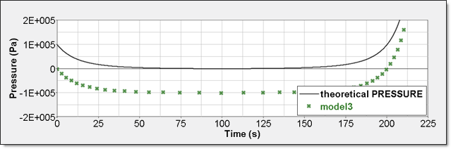
Fig 9: Numerical pressure, model 3: 
Internal energy can be obtained through two different ways. The first one is internal energy density (Eint / V) recorded by element time history (/TH/BRICK). The second one is the internal energy from the global time history because the model is composed of a single element. This numerical internal energy is relative to its initial value; it is shifted with the E0V0 value from the absolute theoretical one and also starts from 0.
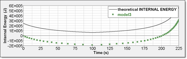
Fig 10: Numerical internal energy, model 3: 
|
Equation of state for a perfect gas is:
Initial internal energy can be introduced:
Which leads to:
P(,E) = ( -1)(1 + )(E0 + E)
Expanding this expression and identifying with polynomial coefficients leads to:
P(,E) = C0 + C1 + (C4 + C5)E
Where,
C0 = C1 = E0 ( - 1)
C4 = C5 = - 1
(1)
|
(2)
|
(3)
|
(4)
|
(5)
|
(6)
|
(7)
|
(8)
|
(9)
|
(10)
|
/MAT/LAW6/mat_ID/unit_ID or /MAT/HYDRO/mat_ID/unit_ID
|
AbsolutePRESSURE_RelativeENERGY
|

|
|
|
|
|
|
|
|
|
|
|
|
|
|
|
|
|
E0( - 1)
|
E0( - 1)
|
0
|
0
|
|
|
0
|
0
|
|
|
|
|
|
|
C4 = - 1
|
C5 = - 1
|
0
|
|
|
|
|
Time History
|
Measure
|
Initial Value
|
Unit
|
/TH/BRICK (P)
|
P
|
P0
|
Pressure
|
/TH (IE)
|
Eint (= E x V0)
|
0
|
Energy
|
/TH/BRICK (IE)
|
Eint / V)
|
0
|
Pressure
|
| 4. | Comparison with Theoretical Result |
Element time history (/TH/BRICK) gives absolute pressure. This result is compared to a theoretical one. Curves are superimposed.
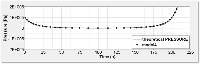
Fig 11: Numerical pressure, model 4: 
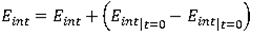
Internal energy can be obtained through two different ways. The first one is internal energy density (ΔEint / V) recorded by element time history (/TH/BRICK). The second one is the internal energy from the global time history 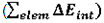 because the model is composed of a single element. This numerical internal energy is relative to its initial value; it is shifted with the E0V0 value from the absolute theoretical one and also starts from 0. because the model is composed of a single element. This numerical internal energy is relative to its initial value; it is shifted with the E0V0 value from the absolute theoretical one and also starts from 0.
Fig 12: Numerical internal energy, model 4: 
|
Sound Speed and Time Step
Material law 6 computes sound speed through the usual expression for fluids:

It can be written in function of :
Then,

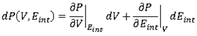
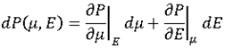
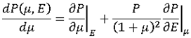
The total differential of P in terms of internal energy E and is:
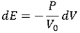
In case of an isentropic transformation (reversible and adiabatic), the change of internal energy Eint with volume V and pressure P is given by:
dEint = -PdV
Using relation which links Eint and E leads to:
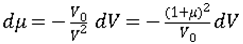
 can be expressed in terms of volume ratio:

its variation in function of the volume change is also:
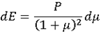
Change in internal energy per unit volume E is then:
Finally, the sound speed is given by:
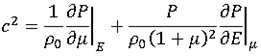
|
(5)
|
This expression computes the sound speed for a given equation of state P( ,E). In the case of perfect gas, it was shown that for each type of formulation (absolute or relative), EOS can be written:
P(,E) = C0 + C1 + (C4 + C5)E
Equation (5) is used to compute sound speed:
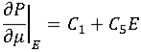
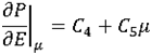
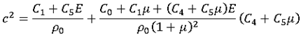
|
(6)
|
This calculation is then applied for each of the four cases.
Numerical Sound Speed vs. Theoretical Expression
|
Case
|
C0
|
C1
|
C4
|
C5
|
c2 from Eq (5)
|
Comparison with theoretical value
|
1
|
0
|
0
|
- 1
|
- 1
|

|
c = cREF
|
2
|
0
|
0
|
- 1
|
- 1
|
|
c = cREF
|
3
|
E0( - 1)
|
E0( - 1)
|
- 1
|
- 1
|
|
c = cREF
|
4
|
E0( - 1)
|
E0( - 1)
|
- 1
|
- 1
|
|
c = cREF
|
For each of the four formulations, the computed sound speed by RADIOSS is the same as the theoretical one. Time step and cycle number are also not affected.


