Flexible Body Input File |

|

|

|

|
|
Flexible Body Input File |

|

|

|

|
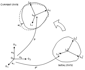
The total displacement field ![]() for every point of a flexible body is obtained from the displacement of a local frame defining the rigid motion of the body and from an additional local displacement field wL corresponding to the small vibrations of the body.
for every point of a flexible body is obtained from the displacement of a local frame defining the rigid motion of the body and from an additional local displacement field wL corresponding to the small vibrations of the body.

(G0, G1, G2, and G3) defines the global frame (e1, e2, and e3).
(L0, L1, L2, and L3) defines an orthonormal local frame.
P is the rotation matrix from (G0, G1, G2, and G3) to (L0, L1, L2, and L3).
The total displacement, u, can thus be expressed as:
![]()
| where | uL0, uL1, uL2, and uL3 are displacements of points L0, L1, L2, and L3 respectively, |
X, Y, and Z are coordinates in the local frame (L0, L1, L2, and L3)
uR is the rigid body contribution to the total displacement
Local displacement is given by a combination of local vibration modes ![]() :
:
WL = ![]() L
L![]()
where, ![]() is the vector of local modal contributions.
is the vector of local modal contributions.
Rigid body displacement uR can also be expressed as a combination of 12 modes:
![]()
where the projection modes ![]() are obtained from the local coordinates:
are obtained from the local coordinates:

The choice of the local frame (L0, L1, L2, and L3) is fully arbitrary. These points do not need to be input explicitly. Their locations define local coordinates and thus, the components of the modes ![]() .
.
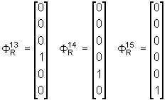
If the flexible body contains elements with rotational DOF, three additional modes must be added to the ![]() family, accounting for the inertia associated with these DOF. The components of these additional modes on each node of the flexible body having rotational DOF are:
family, accounting for the inertia associated with these DOF. The components of these additional modes on each node of the flexible body having rotational DOF are:

In order to solve dynamic equilibrium equations for a flexible body, projected mass and stiffness matrices are required (refer to the RADIOSS Theory Manual for details):
| • | Local mass matrix M projected on modes defining the finite rigid body motion: |
MR = ![]() RT M
RT M![]() R
R
| • | Local mass matrix M projected on local vibration modes: |
ML = ![]() LT M
LT M![]() L
L
| • | Coupled terms corresponding to the cross projection of the local mass matrix M on the finite rigid body modes and on the local modes, expressed in the global frame: |
![]()
where, ![]() is the family of local vibration modes expressed in global coordinates through the rotation matrix P.
is the family of local vibration modes expressed in global coordinates through the rotation matrix P.
The matrix MC is variable with time since the matrix P evolves with the rigid body motion of the flexible body. The former expression is thus split into 9 constant contributions (one for each term of the rotation matrix):
![]()
| where |

The matrices to input are the 9 MCkl matrices.
| • | Local stiffness matrix K projected on local vibration modes: |
KL = ![]() LT K
LT K![]() L
L
If static modes are present in the local projection basis (refer to the RADIOSS Theory Manual), the projected matrix may not be diagonal. However, it may contain a large diagonal block, corresponding to the projection on eigen modes appearing in the basis. The full part and the diagonal part of the matrix are input separately. The shape of the reduced matrix is:

The full part corresponds to ![]() , in which
, in which ![]() is symmetric and
is symmetric and ![]() is rectangular. The diagonal part corresponds to
is rectangular. The diagonal part corresponds to ![]() .
.
| • | Coupled terms corresponding to the cross projection of the local stiffness matrix K on the finite rigid body modes expressed in the local frame and on the local modes: |
![]()
This expression is again split into 9 contributions:
![]()
where ![]()
The matrices to input are now the 9 KCkl matrices.
A flexible body input file is a formatted file whose name is given is the /FXBODY in RADIOSS Starter. It contains several blocks of data which must be input in the right order. Each line beginning with '#' is considered a comment line and is not taken into account.
Example:#FORMAT: (7I8) # Nbmod Nbstat Nbnod Irot Idamp Iblo Ifile 45 15 18 1 0 1 0
Description:
|
Example: #FORMAT: (10I8) # Nodes 21 22 23 24 25 26 27 28 29 30 31 32 33 34 35 36 37 38
Description: The number of nodes in the list must be equal to Nbnod given in Data block 1. The order of nodes in the list is the order in which the sets of components of the projection modes are given in Data blocks 5, 6, and 7. |
Example: #FORMAT: (1P5E16.9) # Mrot11 Mrot12 Mrot13 Mrot21 Mrot22 1.000000000E+00 0.000000000E+00 0.000000000E+00 0.000000000E+00 1.000000000E+00 # Mrot23 Mrot31 Mrot32 Mrot33 Freq 0.000000000E+00 0.000000000E+00 0.000000000E+00 1.000000000E+00 2.049574631E+04
Description:
|
Example:
Description:
|
||||||
Example:#FORMAT: (1P5E16.9) # 1 X Y Z XX YY #FORMAT: (1P1E16.9) # ZZ 0.000000000E+00-1.250000000E+01 0.000000000E+00 0.000000000E+00 0.000000000E+00 0.000000000E+00 0.000000000E+00 1.250000000E+01 0.000000000E+00 0.000000000E+00 0.000000000E+00 0.000000000E+00 ... Description:12 modes
|
Example: Same format as Data block 5
Description:3 modes |
Example: Same format as Data block 5
Description:Nbmod modes |
Example:
Description:Nbmod values are entered, following the order in which the local modes are given. |
||||||||||
Example: Same format as Data block 8
Description:The shape of the matrix to input is (see §2.): [Matsym Matrect]. The dimension of Matsym is Nbstat. The dimensions of Matrect are Nbstat * (Nbmod – Nbstat). The following order for input the terms is followed (for example: Nbmod = 6 and Nbstat = 3):
It corresponds to a skyline storage of the Nbstat first lines of the local reduced stiffness matrix. The number of terms to input is |
Example: Same format as Data block 8
Description:(Nbmod – Nbstat) values are entered, following the order in which the local dynamic modes are given. |
Example: Same format as Data block 8
Description:This is a full symmetric matrix entered using a skyline storage. Column numbering follows the order in which the modes defining the rigid motion are given. The dimension of the matrix is 12, if Irot = 0 or 15, if Irot = 1. Thus, the number of values to input is equal to 78, if Irot = 0 or 120, if Irot = 1. |
Example: Same format as Data block 8
Description:Nine sub-blocks are given, one for each constant contribution MCkl (see §2.). These are rectangular matrices. The number of lines is equal to 12, if Irot = 0 or 15, if Irot = 1. The number of columns is Nbmod. The terms of the matrices are entered line by line. Their number is equal to 12*Nbmod, if Irot = 0 or 15*Nbmod, if Irot = 1. |
Example: Same format as Data block 8
Description:Nine sub-blocks are given, one for each constant contribution KCkl (see §2.). These are rectangular matrices. The number of lines is equal to 12, if Irot = 0 or 15, if Irot = 1. The number of columns is Nbmod. The terms of the matrices are entered line by line. Their number is equal to 12*Nbmod, if Irot = 0 or 15*Nbmod, if Irot = 1. |
Follow the steps below to compute the required data to write a flexible body input file without using RADIOSS:
| 1. | Using a vibration code, compute the mass and stiffness matrices on the model corresponding to the flexible body, then compute the local reduction modes. The modes family can be of any kind (free eigen modes, Craig & Bampton modes, refer to the RADIOSS Theory Manual for further details). |
Orthogonalize the reduction modes with respect to the mass matrix so that the local projected mass matrix is diagonal for matters of efficiency.
| 2. | Choose the locations of the points defining the orthonormal local frame. For example, the origin can be placed at the center of mass if known. Compute the components of the modes defining the finite rigid motion of the flexible body from the coordinates of the nodes in the local frame. Add to the family the modes associated with rotational DOF, if necessary. |
Store the rotation matrix from the local frame to the global frame (it is simply the coordinates of the vectors of the local triedra expressed in the global frame). It is needed to input the initial orientation of the flexible body.
| 3. | Compute the projected matrices MR, ML, and KL. Separately store the full symmetric part and the diagonal part of the local projected stiffness matrix. Compute the maximum eigen frequency of the local dynamic system from ML and KL. |
| 4. | Compute the nine Tkl matrices and transform all the vectors of the local modes family and of the finite rigid body modes family through these matrices. |
Compute the nine mass coupling matrices MCkl and the nine stiffness coupling matrices KCkl.
Use /EIG in RADIOSS Starter to define the part of the model to be included in the flexible body, the type and number of modes to be computed.
In RADIOSS Engine, use /FXINP to create a Flexible Body Input File.
If a set of reduction modes for the flexible body is available, for example from a former experimental analysis or from a vibratory analysis performed with another software, they can be input in /EIG. They will be used to reduce the dimension of the space in which eigenvalues and eigenvectors are searched by RADIOSS and will greatly decrease the time and memory requirements to create the flexible body input file.