Force: FlexModal

Model Element

Description

Force_FlexModal defines a distributed force on a flexible body. The distributed load has two components:

•	A rigid body component that has a tendency to accelerate the flexible body that it is acting on, and,

•	A modal component that has a tendency to deform the flexible body that it is acting on.

Format

<Force_FlexModal

id = "integer"

flex_body_id = "integer"

{

case_idx | case_id = "integer"

scale_expr = "string"

usrsub_param_string = "User(par_1, ... par_N)"

usrsub_dll_name = "string"

[

usrsub_fnc_name = "string"

force_sub = "TRUE" | "FALSE"

]

usrsub_param_string = "User(par_1, ... par_N)"

interpreter = "string"

script_name = "string"

[

usrsub_fnc_name = "string"

force_sub = "TRUE" | "FALSE"

]

}

Attributes

Specifies the element identification number of the Force_FlexModal element. This number should be unique among all Force_FlexModal elements. This parameter is mandatory.

Range: integer > 0

flex_body_id

Specifies the ID of the flexible body on which this force acts. This parameter is mandatory.

Range: integer > 0

case_idx

Specifies the modal load case number that is used to define the shape of the distributed load. Load cases are stored in the XML input deck in a Reference_FlexData modeling element. A separate ModeLoad block within the Reference_FlexData contains all the load cases.

Range: integer >= 0

case_id

Specifies the modal load case ID that is used to define the shape of the distributed load. Load cases are stored in the XML input deck in a Reference_FlexData modeling element. A separate ModeLoad block within the Reference_FlexData contains all the load cases. The difference between an ID and an Index is that indices are required to be contiguous whereas IDs are not.

Range: integer > 0

scale_expr

Specifies an expression evaluated to a scalar quantity. The load case is multiplied by the run-time value of the expression to generate the distributed load acting on the flexible body. Scale_expr can be a constant, a function of time or a function of state. It is required to be continuous.

usrsub_param_string

This keyword defines a list of parameters that are passed from the data file to the user-written subroutine. Use this keyword only when a user-written subroutine is to be defined.

usrsub_fnc_name

This keyword specifies name of the function that contains the definition of the distributed force. This function may be written in Fortran, C, C++ or Python.

usrsub_dll_name

Specifies the path and name of the DLL or shared library containing the user subroutine. MotionSolve uses this information to load the user subroutine in the DLL at run time.

force_sub

A Boolean that specifies whether the user subroutine returns a shape that is to be scaled or the actual force itself.

Range: “TRUE” or “FALSE”

interpreter

Specifies the interpreted language that the user script is written in.

Range: “Matlab” or “Python”

script_name

Specifies the path and name of the user-written script that contains the routine specified by usrsub_fnc_name.

Comments

Force_FlexModal allows you to apply a distributed load on a flexible body. The distributed load may be an aerodynamic load, liquid pressure, a thermal load, an electromagnetic force or any force generating mechanism that is spread out over the flexible body, such as non-uniform damping or visco-elasticity. It may be even be used to model a contact force between two bodies. In the last scenario, Force_FlexModal represents the distributed force acting on one of the flexible bodies involved in the contact.

The force is defined in the modal domain because it is an efficient method for defining the force and calculating its effects. However, this requires that the transformation of the distributed load from the physical domain, where the force is initially defined, to the modal domain be performed in a finite element package.

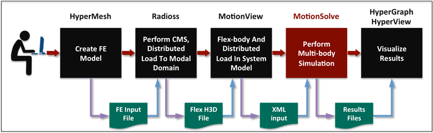
The finite element package responsible for creating the flexible body generates the mode shapes through a process known as component mode synthesis. Since it knows about the modes of the flexible body it is able to transform a NODAL load description to a MODAL load description.

The process for creating distributed forces in HyperWorks is illustrated in Figure 1 below.

force_flexmodal_fig1

Figure-1: The Process For Creating And Analyzing Distributed Loads in HyperWorks

3.	If we define as the mode shapes of the flexible body, and as the Nodal load acting on the flexible body, the equivalent Modal load on the flexible body is defined as:

4.	Since contains only a subset of the full set of modes describing the flexible body, the quantity is lost in the Nodal to Modal conversion. When the CMS method is used correctly, the residual, , is a small quantity.

5.	The transformation from Nodal to Modal basis does not lose the resultant force that acts on the flexible body. The resultant force will tend to provide rigid body motion to the flexible body.

6.	The first six components of the load case or the load vector returned by the user subroutine contain the resultant force. These are defined as follows:

•	1 = Force acting along the X-axis of the LPRF Marker of the flexible body

•	2 = Force acting along the Y-axis of the LPRF Marker of the flexible body

•	3 = Force acting along the Z-axis of the LPRF Marker of the flexible body

•	4 = Torque acting about the X-axis of the LPRF Marker of the flexible body

•	5 = Torque acting about the Y-axis of the LPRF Marker of the flexible body

•	6 = Torque acting about the Z-axis of the LPRF Marker of the flexible body

7.	When the distributed force represents an internal load such as a thermal load or a modal damping force, the first six components (the rigid body components) of the load case are zero.

8.	Force_FlexModal is quite versatile. It provides you with many options for defining the distributed load. These are described below.

•	Option-1: Scale factor defined in a time or state-dependent expression

This method can be used when the modal load shape has been parameterized in terms of quantities available in the multi-body model. In this scenario, you just need to specify the flexible body on which the modal force acts, the load case that you wish to use, and an expression defining the scale factor. The example below illustrates this option.

<Force_FlexModal

id = “101”

flex_body_id = “34”

case_idx = “4”

scale_expr = “Pi*Pitch(1015)*Vx(1015)*Vx(1015)”

•	Option-2: Scale factor defined in a user-subroutine

This method is used when the scale factor is not a simple expression as shown in option-1. In this case, the complex calculations for determining the scale factor may be embedded in a Python script or a compiled Fortran/C function. The example below illustrates how Force_FlexModal is specified in a Python script.

<Force_FlexModal

id = “101”

flex_body_id = “34”

usrsub_param_string = “User(1015)”

interpreter = “Python”

usrsub_fnc_name = “Lift_and_Drag”

script_name = “/Users/MotionSolve/Example/lift.py”

force_sub = “FALSE”

The user subroutine returns two quantities:

o	The load case index

o	The scale factor

MotionSolve uses the above information to apply the distributed load to the flexible body. You are allowed to use SYSFNC and SYSARY to access the instantaneous state of the system and use it to define the scale factor.

•	Option-3: Defining the distributed load shape and scale in a user-subroutine

This method is used when load shape is not available in the Flex-H3D file. This could be for a variety of reasons - one of these is that your finite element solver does not know how to generate a Flex-H3D file. The distributed load is calculated as:

o	, where q is the system state, x the spatial domain over which the distributed load acts and t is the independent variable, time.

The user subroutine returns two quantities:

o	The scale factor, Scale(q,t). You are allowed to use SYSFNC and SYSARY to access the instantaneous state of the system and use it to define the scale factor.

o	The load shape, Shape(x,t). The shape may not be a function of the system states. It can only be a function of the spatial domain and time.

MotionSolve uses the above information to apply the distributed load to the flexible body. The example below illustrates how Force_FlexModal is specified in the case when the user subroutine is written in a compiled language like Fortran, C or C++.

<Force_FlexModal

id = “101”

flex_body_id = “34”

usrsub_param_string = “User(1015)”

usrsub_fnc_name = “Lift_and_Drag”

usrsub_dll_name = “/Users/MotionSolve/Example/lift.so”

force_sub = “FALSE”

<Force_FlexModal

id = “101”

flex_body_id = “34”

usrsub_param_string = “User(1015)”

interpreter = “Python”

usrsub_fnc_name = “Lift_and_Drag”

script_name = “/Users/MotionSolve/Example/lift.py”

force_sub = “FALSE”

•	The results are written to the H3D file and can be visualized using HyperView.

Example

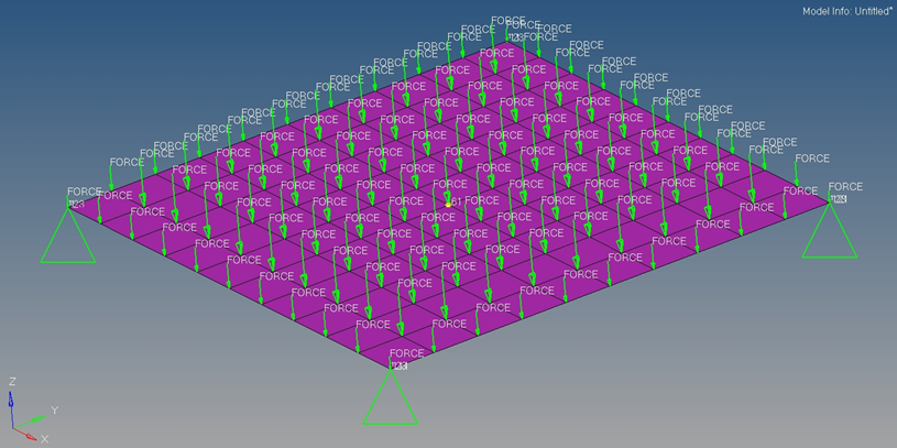
A distributed load acting on a rectangular plate is used as an example to explain how the process illustrated in Figure-1 is implemented. Figure-2 below is the schematic of the system to be analyzed.

force_flexmodal_fig2

Figure-2: The Plate Model

The FE Input file corresponding to the plate and the distributed load is shown in Figure-3.

•	Five interface nodes, four corner nodes (1, 11, 111, 121) and one center node (61) were defined

ASET1 123 111 121 1 11

ASET1 123456 61

•	Point load is applied on all nodes as follows

o	Force of 253.36 N is applied along the negative Z-axis on the corner nodes

o	Force of 506.72 N is applied along the negative Z-axis along the nodes on the edge of the plate

o	Force of 1013.4 N is applied on all the internal nodes

FORCE 7 56 01.0 0.0 0.0 -506.72

FORCE 7 67 01.0 0.0 0.0 -506.72

FORCE 7 78 01.0 0.0 0.0 -506.72

FORCE 7 89 01.0 0.0 0.0 -506.72

FORCE 7 100 01.0 0.0 0.0 -506.72

FORCE 7 11 01.0 0.0 0.0 -253.36

FORCE 7 1 01.0 0.0 0.0 -253.36

FORCE 7 121 01.0 0.0 0.0 -253.36

FORCE 7 111 01.0 0.0 0.0 -253.36

•	Craig-Bampton CMS option is selected with Force applied as LOADSET in CMSMETH card

CMSMETH 8 CB 29

LOADSET BOTH 7

The total number of models calculated for this case will be 48. There will be 4*3 + 1*6 static modes corresponding to the two sets of the ASET1 card defined. One additional static mode corresponding to the LOADSET and 29 dynamic modes as requested in the CMSMETH card.

Number of Modes = 4*3 + 1*6 + 1 + 29 = 48

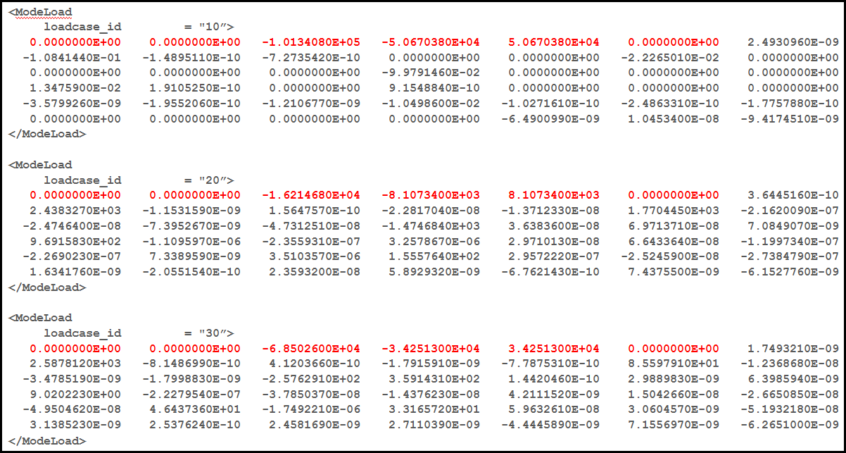
•	The load defined in the LOADSET portion of the CMSMETH card will be projected to the modal space and the modal load information will be written to the Flex-H3D file for MBD solvers to use.

RADIOSS performs its analysis and generates a Flex-H3D file that defines the modal flex body. In addition to the standard CMS data, the Flex-H3D file also contains the distributed load - now defined in the modal domain. MotionSolve reads the Flex-H3D file and places the modal load definition in the ModeLoad section of the Reference_FlexData block. This is shown in Figure 3 below.

force_flexmodal_fig3

Figure-3: The ModeLoad section of Reference_FlexData Block in the XML Input File

The ModeLoad section in the Reference_FlexData block of the MotionSolve XML input file specifies the different load-cases that are available for use. The plate model has 3 load-cases. Each load-case has an ID or an Index.

•	When the ModeLoad data is obtained from an Adams MNF, the load-case index is available.

•	When the data is obtained from a Flex-H3D file, the load-case ID is available. In this example, the load-case was obtained from RADIOSS, so a load-case ID is available for use.

The load-case represents a load shape, it needs to be scaled by a scale factor to obtain the true load on the plate. Each load-case consists of 6+N numbers.

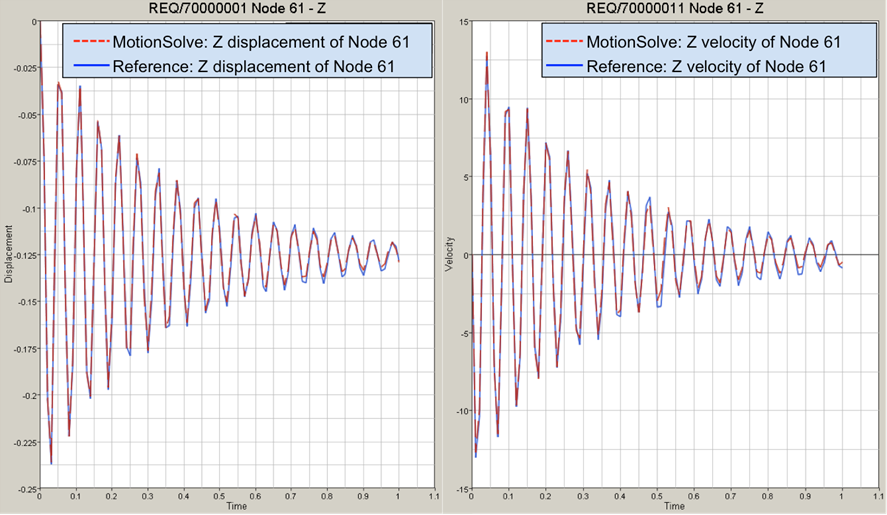
•	The first 6 numbers, highlighted in yellow-red, are the rigid body loads. For the plate model, FZ, TX and TY are non-zero.

•	The next N numbers are the contribution to equations of motion for each mode. The plate was characterized by 42 modes, so N=42 for this example.

Figure 4 shows the z-displacement of Node 61, which is located at the center of the plate. Since a constant load is acting on the plate and damping included, the expectation should be that the oscillations of any node should eventually be dissipated. This is exactly what is seen.

force_flexmodal_fig4

Figure-4: The Z Displacement And Velocity Of Node 61 Compared To A Reference Result

Figure 5 shows the deformation contour of the plate at T=0.45s.

force_flexmodal_fig5

Figure-5: The Z deformation contour of the plate

Model Element
Description
MFORCE defines a distributed force on a flexible body (CMS) in MotionSolve.
Declaration
def MFORCE(id, LABEL= “”, FLEX_BODY=”” , CASE_INDEX= “”, SCALE= "", ROUTINE= "", FUNCTION= "", FORCE= "", INTERPRETER= "", SCRIPT= ""):
Attributes
id	Element identification number (integer>0). This number is unique among all MFORCE elements.
LABEL	The name of the MFORCE element.
FLEX_BODY	Defines the ID of a flex body on which the modal load is applied.
CASE_INDEX	Specifies the modal load case number that is used to define the shape of the distributed load.
SCALE	Specify an expression for the scale factor to be applied to the load case referenced by CASE_INDEX.
ROUTINE	Specify an alternative library and name for the user subroutine MFOSUB.
FUNCTION	Specify user-defined constants that are passed to the MFOSUB.
FORCE	A string that specifies whether the user subroutine returns a shape that is to be scaled or the actual force itself. Set this to USER to specify that the MFOSUB returns the actual force.
INTERPRETER	Specifies the interpreted language that the user script is written in. Valid choices are MATLAB or PYTHON.
SCRIPT	Specifies the path and name of the user written script that contains the routine.
Comments See Force_FlexModal
Example The example below shows a definition of a MFORCE. MFORCE(1,LABEL="MFORCE_1",FLEX_BODY=30102,CASE_INDEX=1,SCALE="1.0+0.2sin(360dtime)+0.1sin(360dtime*3)")

Force: FlexModal

Force: FlexModal

Force: FlexModal

Model Element

Description

Format

Attributes

Comments

Example

Model Element

Description

Declaration

Attributes

Specify an expression for the scale factor to be applied to the load case referenced by CASE_INDEX.

Comments

See Force_FlexModal

Example