Composite materials have become popular in the application of a variety of structures. The need for innovative designs has posed a great challenge. This tutorial discusses the optimization-driven design approach of an open-hole tension specimen using OptiStruct.
The design takes a three-phased approach:
|
|
Concept design synthesis
Free-size optimization identifies the optimal ply shapes and locations of patches per ply orientation.
|
|
|
Design fine tuning
Size optimization identifies the optimal thicknesses of each ply bundle.
|
|
|
Ply stacking sequence optimization
Shuffling optimization obtains an optimal stacking sequence.
|
The process expands upon three important and advanced optimization techniques; free-size optimization, size optimization and ply stacking sequence optimization. By stringing these three techniques together, OptiStruct offers a unique and comprehensive process for the design and optimization of composite laminates. The process is automated and integrated in HyperWorks by generating the input data for a subsequent phase automatically from the previous design phase.
Together with these steps, an initial and final analysis will be utilized to determine the baseline and final characteristics of the designed part.
Problem Definition
The composite design optimization methodology presented within this tutorial was developed to solve very complex composite design optimization problems. The methodology breaks down the complex composite design optimization problem, which is not solvable by itself, into several simpler composite design optimization problems, which are solvable by themselves. The cumulative solution to each of the simpler composite design optimization problems provides a solution to the complex design optimization problem. This process of breaking down complex problems into several simpler problems is consistent with the engineering method.
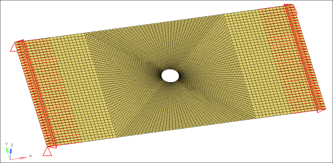
Model overview
Initial Model Setup and Baseline Analysis
The following set of steps completes the analysis setup of the initial model and provides a baseline analysis for comparison with the final optimized structure.
Step 1: Load the OptiStruct user profile and open the model into HyperMesh
| 2. | Select OptiStruct in the User Profiles dialog and click OK. This loads the user profile. It includes the appropriate template, macro menu, and import reader, paring down the functionality of HyperMesh to what is relevant for generating models OptiStruct. |
User Profiles can also be accessed from the Preferences menu on the toolbar.
| 3. | Select the Open Model file toolbar icon  |
| 4. | Select the oht_analysis.hm file you saved to your working directory from the optistruct.zip file. Refer to Accessing the Model Files. |
| 5. | Click Open. The oht_analysis.hm database is loaded into the current HyperMesh session. |
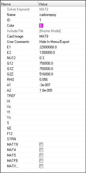
Step 2: Create a new material for carbon epoxy
| 1. | Right-click in the Model browser and select Create > Material to create a new material. |
| 2. | In the Entity Editor, for Name, enter carbonepxy. |
| 3. | Set the value for Card Image to MAT8 and enter the values shown below: |
Step 3: Create a new element set containing the initial shape of each ply
| 1. | Right-click in the Model browser and select Create > Set to create a new set. |
| 2. | In the Entity Editor, for Name, enter ply_shape. |
| 3. | Set the value for Card Image to SET_ELEM. |
| 4. | Click Entity IDs and click the yellow Elements entity selector. |
| 5. | Use the yellow elems entity selector to select all of the elements in the model. |
| 6. | Click proceed to continue. |
Step 4: Create the basic plies for the analysis
| 1. | Right-click in the Model browser and select Create > Ply to create a new ply. |
| 3. | Set Material type to ORTHOTROPIC. |
| 4. | Set Material to carbonepxy. |
| 5. | Set Thickness to 0.1, and Orientation to 0. |
| 6. | Switch the Shape drop-down selector to Set, and use the yellow Set entity selector to select the ply_shape set created in the previous step. |
| 7. | Ensure that Output results is checked. |
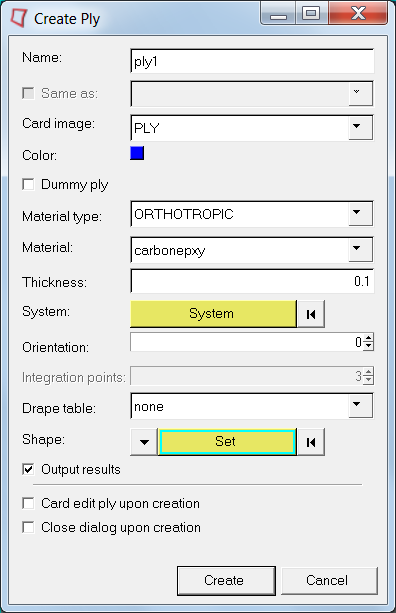
| 9. | Using these steps, create three more plies: ply2 with orientation 90, ply3 with orientation 45, and ply4 with orientation -45. |
| 10. | Close the dialog box to continue with the exercise. |
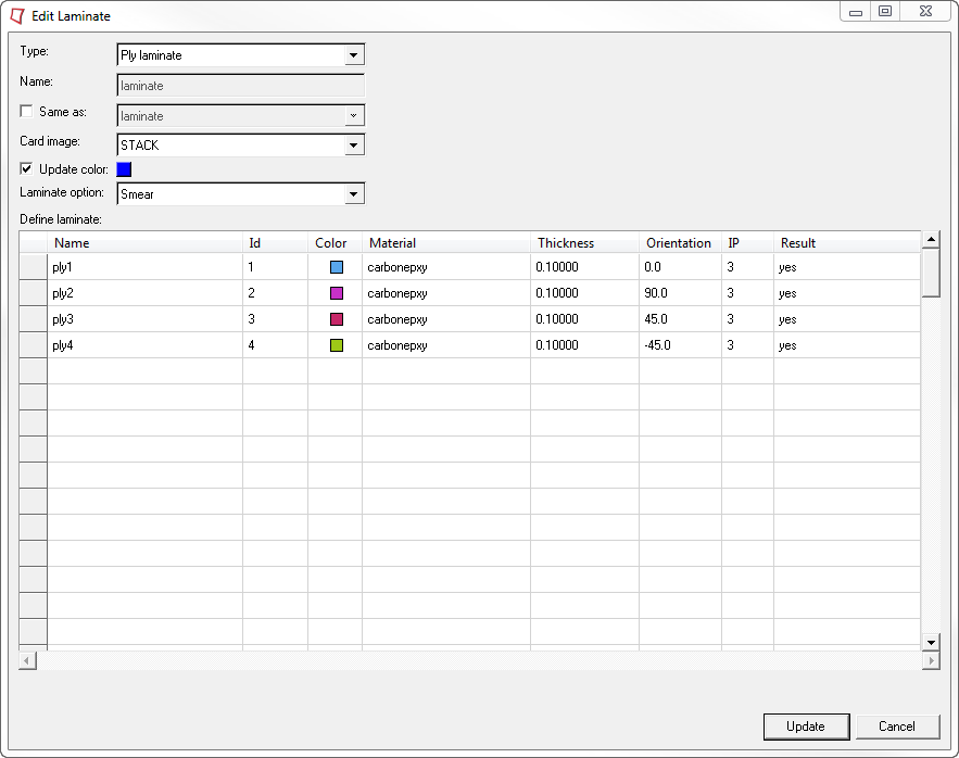
Step 5: Create the laminate for the analysis
| 1. | Right-click in the Model browser and select Create > Laminate to open the create laminate dialog box. |
| 3. | Set Card image to STACK. |
| 4. | Set Laminate option to Smear. |
| 5. | In the Define laminate section, select ply1 for the first row, with each successive ply on a consecutive row. Leave all other parameters set as default and click Create to create the laminate. |
| 6. | Close the dialog box to continue with the exercise. |
Step 6: Create a property and assign it to all elements in the model
| 1. | Right-click in the Model browser and select Create > Property to create a new property and load it into the Entity Editor. |
| 2. | For Name, enter laminate_property. |
| 3. | Set Card Image to PCOMPP. |
| 4. | In the Model browser, right-click on the laminate_property property and select Assign. |
| 5. | Use the yellow elems entity selector to select all elements in the model and click proceed to continue. |
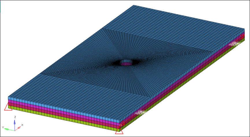
Step 7: Review the model
| 1. | Select the element visualization icon  and change the mode to 2D Detailed Element Representation using the drop-down selector. and change the mode to 2D Detailed Element Representation using the drop-down selector. |
This will thicken all shells in the model to their total thickness, displaying them as 3-dimensional representations of their thicknesses.
| 2. | Click the Layers icon  and select Composite Layers. and select Composite Layers. |
This separates the view into individual plies.
| 3. | To assist in determine which plies are which in the layup, change the element color mode to By Prop  . . |
This represents each of the plies in the model according to the color of its ply as shown in the Model browser. If all of the plies in the model are the same color, change the ply colors in the Model browser so that each is different to help differentiate the plies in the graphics area.
Step 8: Create control cards to set the request and output parameters
| 1. | In the control cards panel on the Analysis page, enter the GLOBAL_OUTPUT_REQUEST panel. |
| 2. | Check the box for CSTRAIN. Set EXTRA(1) to MECH and OPTION(1) to ALL. |
| 3. | Check the box for DISPLACEMENT. Set OPTION(1) to ALL. |
| 4. | Check the box for STRESS. Set OPTION(1) to NO. |
This requests that NO homogeneous stress be output. This control card output must be explicitly added as a request since homogeneous stress is output by default. In turning it off, the values will not be calculated by the solver for output.
| 5. | Click return to return to the control cards panel. |
| 6. | Enter the OUTPUT panel. Set number_of_outputs to 2. |
| 7. | For the first OUTPUT, set KEYWORD to HTML and OPTION to NO. |
This turns off HTML output for all analyses and optimizations which have this keyword combination.
| 8. | For the second OUTPUT, set KEYWORD to H3D and FREQ to FL. |
This request that OptiStruct’s .h3d output file be output at the first (F) and last (L) iteration. For analysis, this does not matter, but for optimization it applies when you get to the optimization runs.
| 9. | Click return twice to return to the Analysis page. |
Step 9: Run the baseline analysis
| 1. | Enter the OptiStruct panel on the Analysis page. |
| 2. | Ensure that export options is set to all and run options is set to analysis. |
| 3. | Click OptiStruct to export the model and run the baseline analysis as oht_analysis.fem. |
Step 10: Post-process the baseline analysis in HyperView
| 1. | When the run is complete, click HyperView in the OptiStruct panel to load the results into HyperView. |
| 2. | Enter the Contour panel  . . |
| 3. | Set Result type to Composites Strains(Mech) (s) and subtype to Normal X Strain. |
| 4. | To view the individual strain contributions from any one ply, select the appropriate ply name in the Layers drop-down. |
Step 11: Return to HyperMesh and deactivate the composite visualization enhancements
| 1. | Return to the HyperMesh client by using Delete Page icon  to close the HyperView session. to close the HyperView session. |
| 2. | Click the element visualization icon on the button bar to return the mode to 2D Traditional Element Representation using the drop-down selector. |
| 3. | Use the Layers  drop-down selector to select Layers Off. drop-down selector to select Layers Off. |
| 4. | Return element color mode to By Comp. |
Phase 1 – Concept Design Synthesis (free-size optimization)
In free-size optimization, the thickness of each designable element is defined as a design variable. Applying this concept to the design of composites implies that the design variables are the thickness of each ‘Super-ply’ (total designable thickness of a ply orientation) per element.
The following optimization setup is defined in the concept design phase to identify the stiffest design for the given fraction of the material. To obtain more meaningful results, manufacturing constraints are incorporated and carried through all design phases automatically.
Objective:
|
Minimize the compliance of the load case.
|
Constraints:
|
Volume fraction < 0.3
|
Design variables:
|
Element thicknesses of each ply orientation.
|
Manufacturing constraints:
|
| • | Ply percentage for the 0s no more than 80% exist. |
| • | The manufacturable ply thickness is 0.1. |
| • | A balance constraint that ensures an equal thickness distribution for the +45s and -45s. |
|
Step 1: Create the design variables for free-size optimization
| 1. | From the Analysis page, enter the optimization panel. |
| 2. | Click free size to enter the free-size optimization panel. |
| 3. | On the create subpanel, enter free-size in the desvar= field. |
| 4. | Click the switch under type and select STACK. |
| 5. | Click the highlighted laminate, select laminate, and click return. |
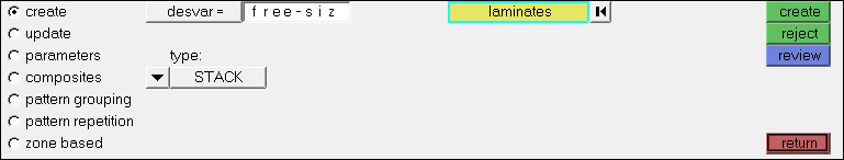
Figure 1: Field entries for the free-size panel
| 6. | Verify that the fields in the create subpanel match the fields shown above and click create. |
The design variable free-size is created for the free-size optimization. The manufacturing constraints on ply percentage and ply balance will be defined next.
| 7. | Go to the composites subpanel. Make sure free-size is selected as the design variable. |
| 8. | Click edit and enter the DSIZE panel to define the manufacturing constraints on ply percentage, ply balance, and ply drop-off. |
| 9. | Check the box in front of PLYPCT. |
| 10. | Set Ply Percentage Options to BYANG. |
| 11. | In the DSIZE_NUMBER_OF_PLYPCT= field, enter the value of 2. |
Two PLYPCT continuation lines are added to the DSIZE data entry.
| 12. | In the first PLYPCT row, for PANGLE(1) enter 0, PPMIN(1) enter 0.2, and PPMAX(1) enter 0.7. |
| 13. | In the next PLYPCT row, for PANGLE(2) enter 90, PPMIN(2) enter 0.2, and PPMAX(2) enter 0.7. |
These values constrain the zero- and ninety-degree plies to between twenty and seventy percent of the total thickness of the laminate for any element in the design space.

Figure 2: DSIZE data entry fields for the PLYPCT cards
| 14. | Check the box in front of BALANCE. |
| 15. | Set Balance Constraints Options to BYANG. |
| 16. | In the DSIZE_NUMBER_OF_BALANCE= field, enter the value of 1. |
A BALANCE continuation line is added to the DSIZE data entry.
| 17. | In the BALANCE row, for BANGLE1, enter 45 and for BANGLE2, enter -45. |

Figure 3: DSIZE data entry fields for the BALANCE card
| 18. | Check the box in front of PLYDRP. |
A PLYDRP continuation line is added to the DSIZE data entry.
| 19. | Set Ply Drop-off Options to All. |
| 20. | In the DSIZE_NUMBER_OF_PLYDRP= field, enter the value of 1. |
| 21. | In the PLYDRP row, for PDTYP(1) enter PLYSLP and for PDMAX(1) enter 0.33. |

Figure 4: DSIZE data entry fields for the PLYDRP card using the PLYSLP method
| 22. | Click return to go back to the composites subpanel. |
| 23. | Click update > return and go back to the optimization panel. |
Step 2: Create the responses
| 2. | In the response= field, enter volfract. |
| 3. | Set the response type to volumefrac and that the sub-type is set to total. |
| 5. | In the response= field, enter compliance. |
| 6. | Set the response type to compliance. |
| 7. | Make sure that total is selected and the toggle is set to no regionid. |
| 9. | Click return to go back to the optimization panel. |
Step 3: Define constraints for optimization
| 1. | Select the dconstraints panel. |
| 2. | In the constraint= field, enter volfract. |
| 3. | Click response= and select volfract. |
| 4. | Activate upper bound= and enter a value of 0.3. |
Step 4: Define the objective function
| 1. | Select the objective panel. |
| 2. | For optimization type, select min. |
| 3. | Click response= and select compliance. |
| 4. | Click the loadstep entity selector and select the loadstep nx_step. |
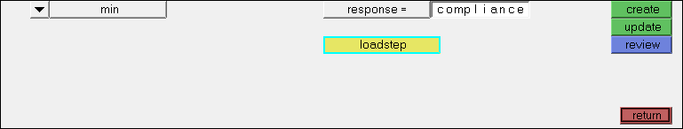
Figure 5: Optimization Objective Panel (Compliance)
| 6. | Click return twice to go back to the Analysis page. |
Step 5: Add an output request to output the next optimization step
The output control on composite strain and stress results are defined here. OUTPUT,FSTOSZ (free size to size) is used to output a ply-based input deck for size optimization.
| 1. | From the Analysis page, select control cards. |
| 3. | In the OUTPUT panel, enter 3 as the number_of_outputs. |
| 4. | On the third line, under KEYWORD, select FSTOSZ and for FREQ, select YES. |
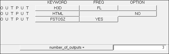
Figure 6: Requesting the free-size to size (FSTOSZ) optimization output file for Phase 2.
With this keyword, OptiStruct automatically generates a sizing model after free-size optimization.
| 5. | Click return twice to go back to the Analysis page. |
| 6. | Save the file as oht_opti_ph1.hm. |
Step 6: Submit the free-size optimization job
| 1. | From the Analysis page, select the OptiStruct panel. |
| 2. | Click save as following the input file field. |
| 3. | Select the directory where you would like to write the OptiStruct model file and enter the name for the model, oht_opti_ph1.fem, in the File name field. |
The name and location of the oht_opti_ph1.fem file displays in the input file field.
| 5. | Toggle export options to all. |
| 6. | Toggle run options to optimization. |
| 7. | Toggle memory options to memory default. |
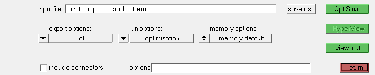
Figure 7: OptiStruct Panel
| 8. | Click OptiStruct. This launches OptiStruct to run the job. |
If the job was completed successfully, new results files can be seen in the directory from which oht_opti_ph1.fem was saved.
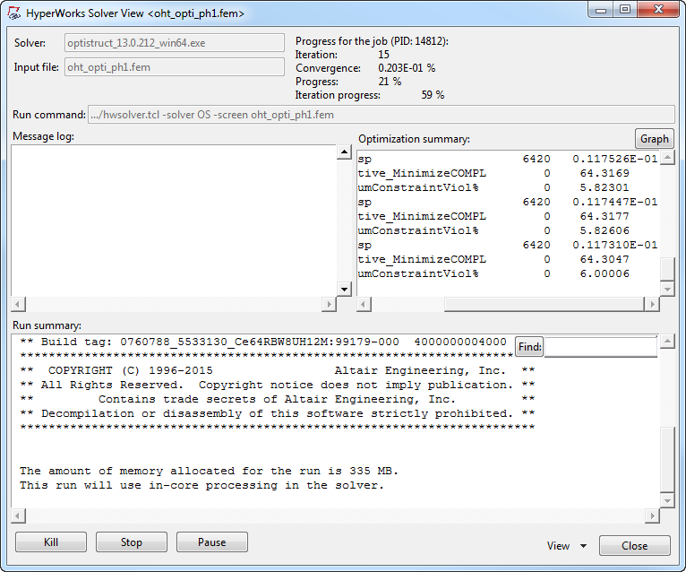
Figure 8: The HyperWorks Solver View window
A few default files which will be written to your directory are:
oht_opti_ph1_s1(2).h3d
|
Hyper 3D binary results file, with the static analysis results of both subcases.
|
oht_opti_ph1_des.h3d
|
Hyper 3D binary results file, with free size optimization results.
|
oht_opti_ph1.out
|
An ASCII output file contains specific information on the model setup, compute time information, etc. Review this file for warnings and errors.
|
oht_opti_ph1_sizing.*.fem
|
A ply-based sizing optimization input file generated during free-sizing phase. This resulting deck contains PCOMPP, STACK, PLY, and SET cards describing the ply-based composite model, as well as DCOMP, DESVAR, and DVPREL cards defining the optimization data. The * sign represents the final iteration number.
|
oht_opti_ph1_sizing.*.inc
|
An ASCII include file contains the same ply-based modeling and optimization data as in the input deck. The * sign represents the final iteration number.
|
Step 7: View the element thickness results
| 1. | When the job is complete, click HyperView from the OptiStruct panel. |
This launches the HyperView client from HyperMesh Desktop and opens the session file oht_opti_ph1.mvw which contains three pages with the results from two H3D files (click Close in the Message Log window):
Page 2 – optimization results in oht_opti_ph1_des.h3d
Page 3 – analysis results of subcase 1 in oht_opti_ph1_s1.h3d
Note: If opening these files from standalone HyperMesh, the page numbers will be decremented.
| 2. | On the page with the results for oht_opti_ph1_des.h3d (open file name is shown in the upper right corner by default), go to the Contour panel and select the plot options. |
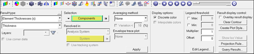
Figure 9: Contour panel plot options (free-size optimization results)
| 3. | In the Results browser, select the last iteration in the Load Case and Simulation Selection drop-down. |
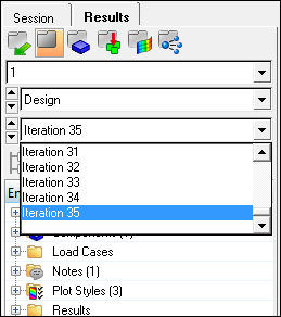
Figure 10: Selecting the final iteration
| 4. | Click Apply and then XY Top Plane View  to view the results in the X-Y plane. to view the results in the X-Y plane. |
The element thickness results from the free-size optimization are shown in the image below. The regions indicated in red or in colors tending towards red (from the legend) can be interpreted as thicker regions, while those in blue or tending towards blue are thinner regions. The contour plot indicated above is the total thickness distribution that includes contributions from each ply orientation, i.e. a thickness contribution from the 0s, +/-45s and the 90s. It also indicates the shape and layout of plies per orientation as can be seen in the ply thickness plot.
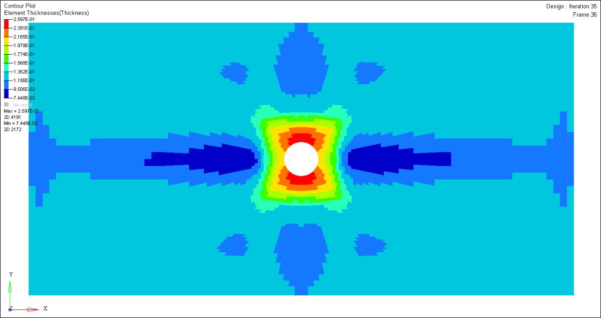
Figure 11: Element thicknesses contour plot after free-size optimization
Step 8: View the ply thickness results
| 1. | From the Contour panel, select Ply Thicknesses (s) as the Result type. Select the other plot options shown below. |
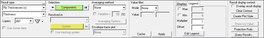
Figure 12: Ply Thicknesses contour plot
| 2. | Select the last iteration in the Load Case and Simulation Selection drop-down. |
The thickness distribution of 0 degree super ply is generated. It represents the ply shapes and patch locations of the 0 degree ply bundles.
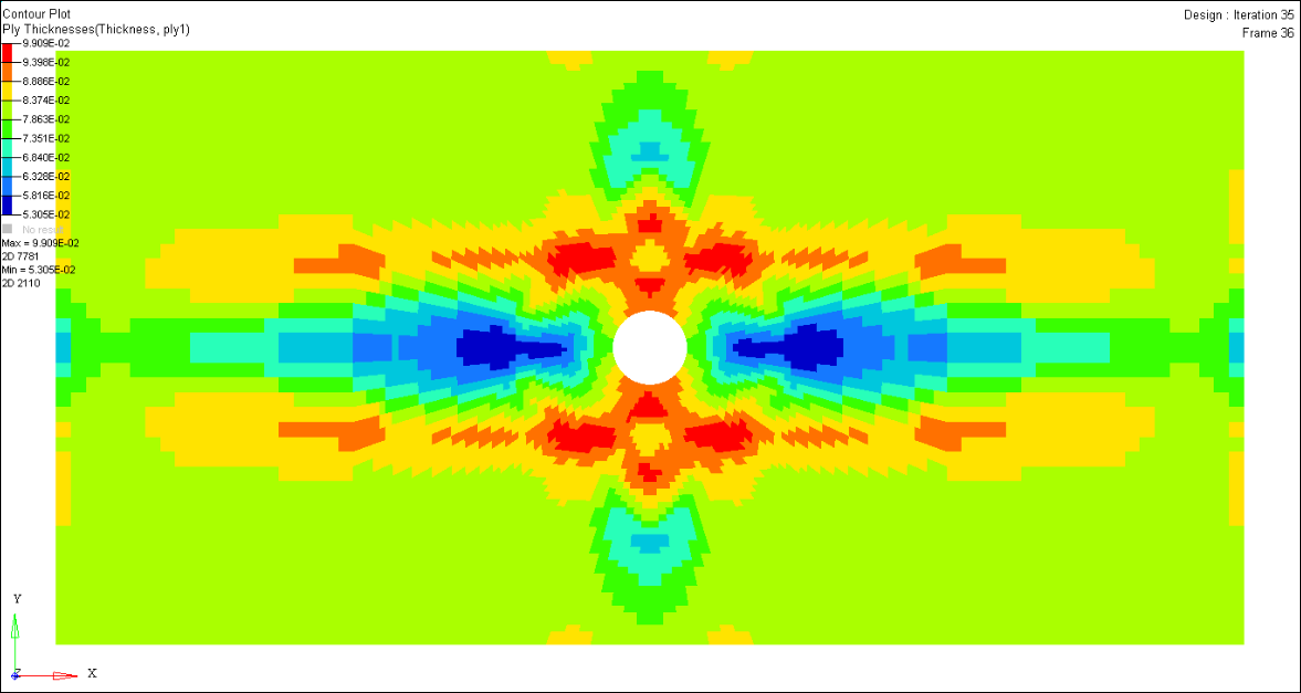
Figure 13: Ply Thickness Contour plot of the 0 degree super-ply
| 4. | Repeat step 1 through 3 to create the ply thickness contours for super-ply 2 (45°), ply 3 (-45°), and ply 4 (90°) by selecting Layers 2, 3 and 4, respectively in the Contour panel. |
| 5. | The figures below represent the ply shapes and patch locations of +/-45 and 90° ply bundles. Due to the balance constraint applied, the thickness distribution of the +45° and the -45° super ply are the same. |
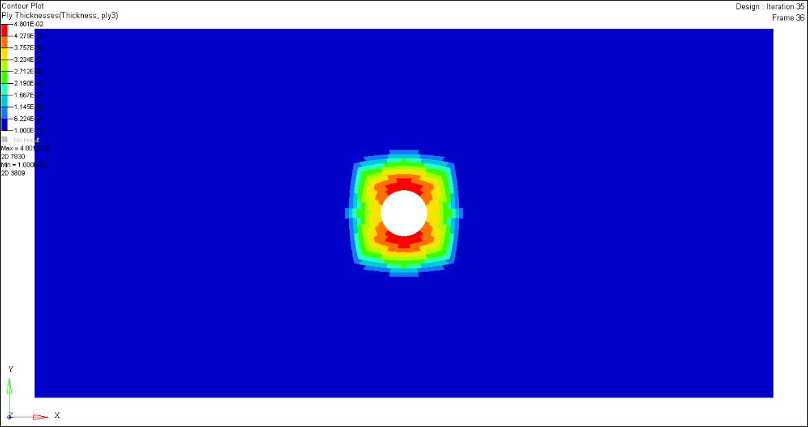
Figure 14: Ply Thickness Contour plot of the -45/+45 degree super-plies
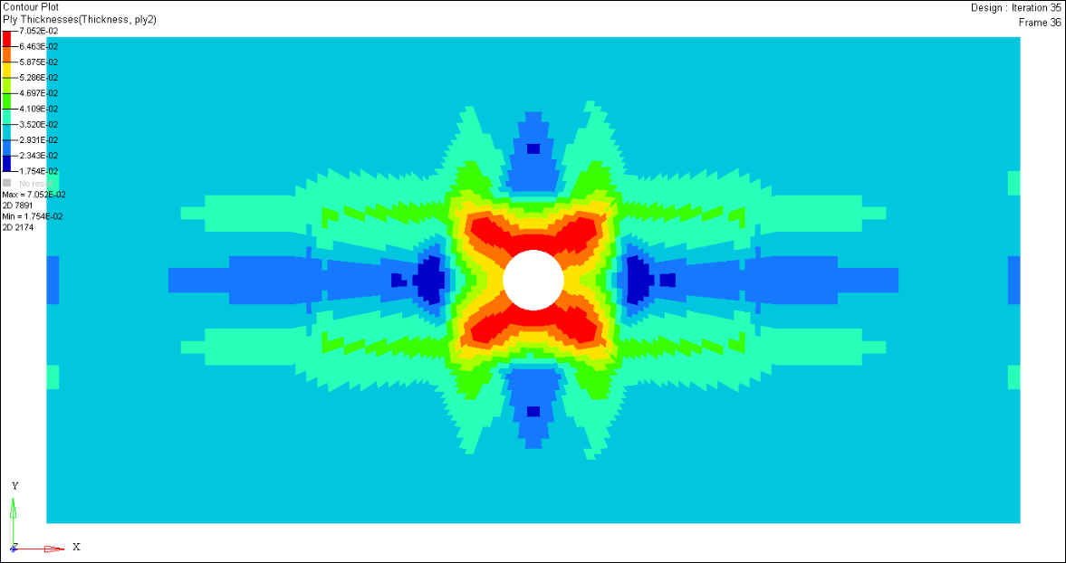
Figure 15: Ply Thickness Contour plot of the 90 degree super-ply
Step 9: View the ply bundles in the optimization result fem
The optimized ‘Super-ply’ thickness is subsequently represented as ‘Ply Bundles’. Four ply bundles per fiber orientation (Super ply) are output by default, based on an intelligent algorithm in OptiStruct. These ply bundles represent the shape and location of the plies per fiber orientation through element sets. In this case, a total of 16 ply bundles are created after free size optimization converges: plies 1 through 4 represent the ply bundles for 0 degree super-ply; plies 5 through 8 represent ply bundles for 90 degree super-ply; plies 9 through 12 represent ply bundle +45 degree super-ply; and applies 13 through 16 represent ply bundles for -45 degree super-ply.
| 1. | Return to the HyperMesh session by deleting the HyperView client windows. |
| 2. | Open a new model by clicking the New Model icon  . . |
| 3. | Click the Import Solver Deck panel toolbar icon  . . |
| 4. | The File type is OptiStruct. |
| 5. | Click the open file icon  in the File field. in the File field. |
| 6. | Select the oht_opti_ph1_sizing.*.inc file, located in the same directory where the file oht_opti_ph1.fem is saved. |
| 7. | Click Import to import the model into session. |
| 8. | Turn the display off for all the load collectors: go to the Model browser, right-click on LoadCollector and select Hide. |
| 9. | Using the Model browser, hide all plies. |
| 10. | To review the plies, expand the Ply tree in the Model browser and activate the mesh view icon for each ply individually as shown below. |
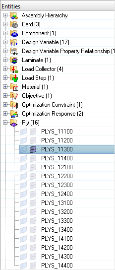
Figure 16: Model browser view showing ply 11300 selected (Laminate 1, Ply 1, Shape 3)
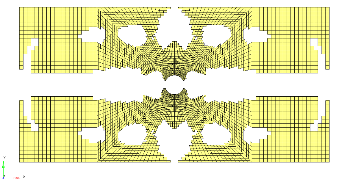
Figure 17: Graphics Area view of ply 11300 (Laminate 1, Ply 1, Shape 3)
The shapes of the plies as indicated through the element set can be used as-is in design Phase 2, or modified easily by updating the element sets in HyperMesh or using ply smoothing to improve the manufacturability. Ply smoothing operations are shown in the next section.
Step 10: Use OSSmooth to perform ply smoothing operations on the model
Ply smoothing is an automated method to further reduce the ply shapes into more manufactural ply shapes. Although ply smoothing significantly improves the ply shapes for manufacturability, often it is still necessary to manually edit the ply shapes after this step.
| 1. | In the Post page, enter the OSSmooth panel. |
| 2. | Click the file selection icon to set Select model to oht_opti_ph1_sizing.35.fem. |
| 3. | Change the mode from Geometry to PLY Shape. |
| 4. | Use the file icon to set the output file selection to the original location with the name of oht_opti_ph1_sizing.35.smoothed.fem. |
| 5. | Set smooth iterations: to 20. |
| 6. | In small region: deselect checkboxes for split disconnected and create geometry. |
| 7. | Set area ratio: to 0.010. |
| 8. | Click OSSmooth to run the analysis to smooth the model. |
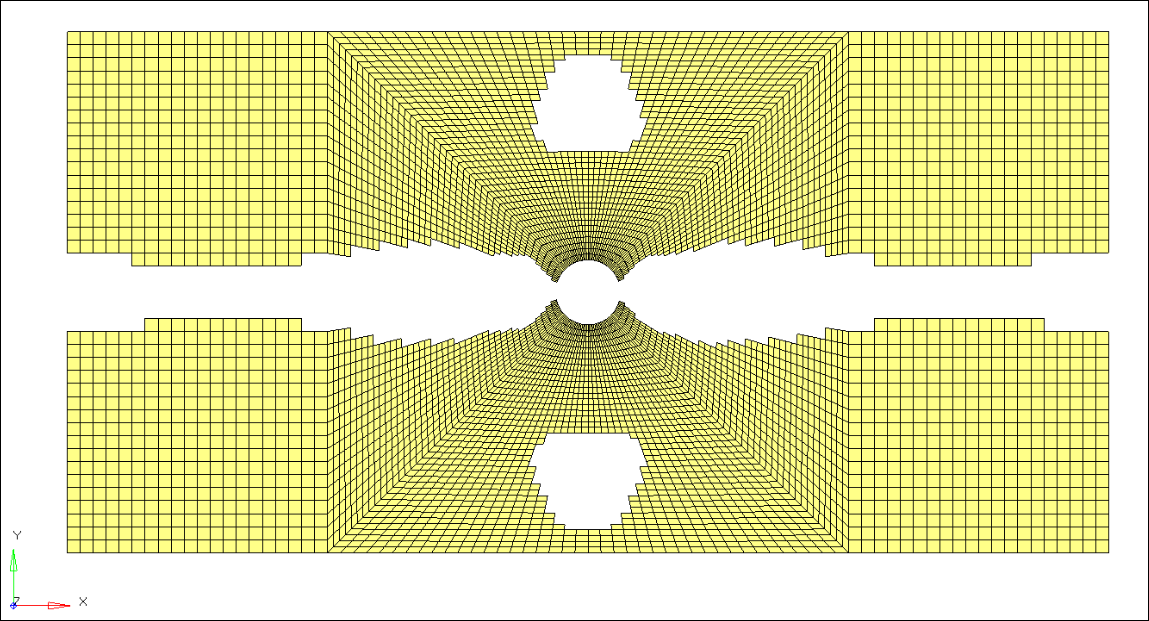
Figure 18: Graphics Area view of ply 11300 after smoothing operations in OSSmooth (Laminate 1, Ply 1, Shape 3)
Phase 2 – Design Fine Tuning (size optimization)
In the second design phase, a size optimization is performed to fine tune the thicknesses of the optimized ply bundles from Phase 1. To ensure that the optimization design meets the design requirements, additional performance criteria on may be incorporated into the problem formulation. These new criteria will be fiber strain, matrix strain, and mass.
The following is the modified optimization setup:
Design variables:
|
Ply thicknesses, which have been defined in the size input deck from Phase 1
|
Objective:
|
Minimize the total mass
|
Constraints:
|
| • | Fiber Strain < 9000 με (microstrain) |
| • | Matrix Strain < 7000 με (microstrain) |
|
Manufacturing constraints previously applied are preserved and transferred to the DCOMP card.
Step 1: Save the model as oht_opti_ph2.hm
Step 2: Review and edit the size design variables
| 1. | From the optimization panel, click size. |
| 2. | Click review and select autoply. |
| 3. | Set the initial value= to 0.04, the thickness of four plies. |
| 4. | Set the upper bound to 0.2, set the lower bound to 0.0. |
| 5. | Click update to update the design variable. |
| 6. | Repeat steps 2.3 through 2.5 on each of the size design variables to update the bounds and starting value for each. |
| Note: | The DESVARs have the same ID numbers as the design variable property relationship (DVPREL) that they relate to. These ID numbers also refer to the plies created in the previous optimization – in this way, they can easily be cross-referenced. |
Step 3: Edit the manufacturable thickness and initial value of each ply
| 1. | In the Model browser, select all plies as shown below. |
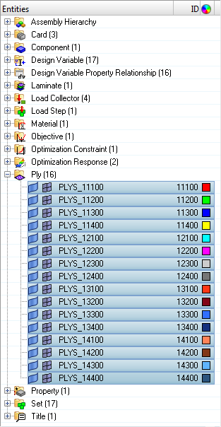
Figure 19: A view of the Model browser showing all plies selected
| 2. | In the Entity Editor, set TMANUF to 0.01 and Thickness to 0.04. |
This changes the values for all plies simultaneously.
Step 4: Update the laminate calculation type
| 1. | In the Model browser, right-click and select Laminate > laminate > Edit. |
| 2. | In the laminate edit dialog box, set Laminate option to Symmetric smear. |
The laminate option defines the laminate behavior. In this case SMEAR theory is used to define the laminate behavior; that is the A-matrix is calculated exactly since it is stacking sequence independent, the D-matrix is calculated as AT2/12, and finally the B-matrix is set to zero. Adding the Symmetric option to the SMEAR theory just assures a symmetric laminate will be output by adding/removing 2 plies at a time vs. 1 ply at a time.
Step 5: Delete the existing responses, constraints, and objective
| 1. | Right-click in the Model browser, and select Optimization Response > Delete. |
| 2. | HyperMesh asks you to confirm the delete. Click Yes to continue. |
When responses are deleted in HyperMesh, all constraints and objectives which depend on those responses are deleted.
Step 6: Create the new responses for size optimization
The responses of volume, natural frequency, and composite strain are created for size optimization.
| 1. | Click optimization and then click responses. |
| 2. | In the response= field, enter fiber_e. |
| 3. | Set the response type to composite strain, set the component to mechanical, change the entity selector to plies, and use the plies entity selector to select all plies in the model. |
| 4. | Set the response component to normal 1, and check the box for all plies. |

Figure 20: The fiber mechanical strain response
| 5. | Click create to create the new response. |
| 6. | In the response= field, enter matrix_e. |
| 7. | Set the response type to composite strain, set the component to mechanical, set the entity selector drop-down to plies, and use the plies entity selector to select all plies in the model. |
| 8. | Set the response component to normal 2, and check the box for all plies. |
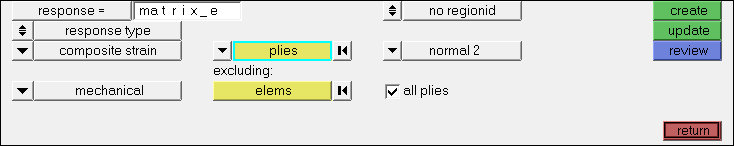
Figure 21: The matrix mechanical strain response
| 9. | Click create to create the new response. |
| 10. | In the response= field, enter mass. |
| 11. | Set the response type to mass, set the type to total. |
| 13. | Click return to go back to optimization panel. |
Step 7: Create optimization constraints
The responses of fiber and matrix strain are defined as the optimization constraints.
| 1. | From the optimization panel, click dconstraint. |
| 2. | For constraint=, enter fiber_e. |
| 3. | Click response= and select fiber_e. |
| 4. | Activate upper bound and enter 0.009. |
| 5. | Click the highlighted loadsteps and select the loadcase nx_step. |
| 7. | Repeat steps 7.2 through 7.6 to create constraint matrix_e on response matrix_e for loadstep nx_step with an upper bound of 0.007. |
| 8. | Click return to go back to the optimization page. |
Step 8: Create objective function for the optimization
| 2. | Select min as the optimization type. |
| 3. | Click response= and select mass. |
| 5. | Click return to go back to the optimization page. |
Step 9: Edit the composite size design variable to update the manufacturing constraints
| 1. | From the Analysis page, select composite size. |
| 2. | Click review and select the free-size design variable. |
This DESVAR has been carried over from the previous optimization as a size optimization with manufacturing constraints preserved from the original optimization.
| 3. | On the parameters subpanel, toggle minimum thickness to activate it and enter a value of 0.04. |
| 4. | Click edit and review the manufacturing constraints to ensure that PLYPCT is set to restrict 0 and 90-degree plies to between 0.2 and 0.7, BALANCE is set to 45 and -45 degree plies, and PLYDRP is still set to TOTAL with a PDMAX of 0.33. |
| 5. | Click return to keep these parameters. |
| 7. | Click return twice to return to the Analysis page. |
Step 10: Define the output request for shuffling deck
The output control on composite strain and stress results defined in the previous phase are carried over automatically. OUTPUT,SZTOSH (sizing to shuffling) writes a ply stacking optimization input deck.
| 1. | From the Analysis page, select control cards. |
| 2. | Go to the OUTPUT panel. |
| 3. | Change the final keyword, FSTOSZ, to SZTOSH and YES for FREQ. |
| 4. | Click return twice to go back to the Analysis page. |
Step 11: Submit the size optimization job
| 1. | From the Analysis page, click OptiStruct. |
| 2. | Click OptiStruct to launch OptiStruct and run the optimization. |
If the job was completed successfully, new results files can be seen in the same directory where oht_opti_ph2.fem was saved.
A few default files are:
oht_opti_ph2_s1.h3d
|
Hyper 3D binary results file, with the analysis results of each subcase.
|
oht_opti_ph2_des.h3d
|
Hyper 3D binary results file, with size optimization results.
|
oht_opti_ph2.out
|
An ASCII output file containing specific information on the model setup, compute time information, etc. Review this file for warnings and errors.
|
oht_opti_ph2_shuffling.*.fem
|
A ply stacking optimization input deck. The DESVAR and DVPREL cards from the previous stage are removed, and a bare DSHUFFLE card is introduced. The * sign represents the final iteration number.
|
oht_opti_ph2_shuffling.*.inc
|
An ASCII include file containing ply stacking optimization data.
|
Step 12: View the thickness results in HyperView
| 1. | Click HyperView in the OptiStruct panel when the run has completed. |
| 2. | Follow the instructions in Step 7 from Phase 1 to create the Thickness contour. |
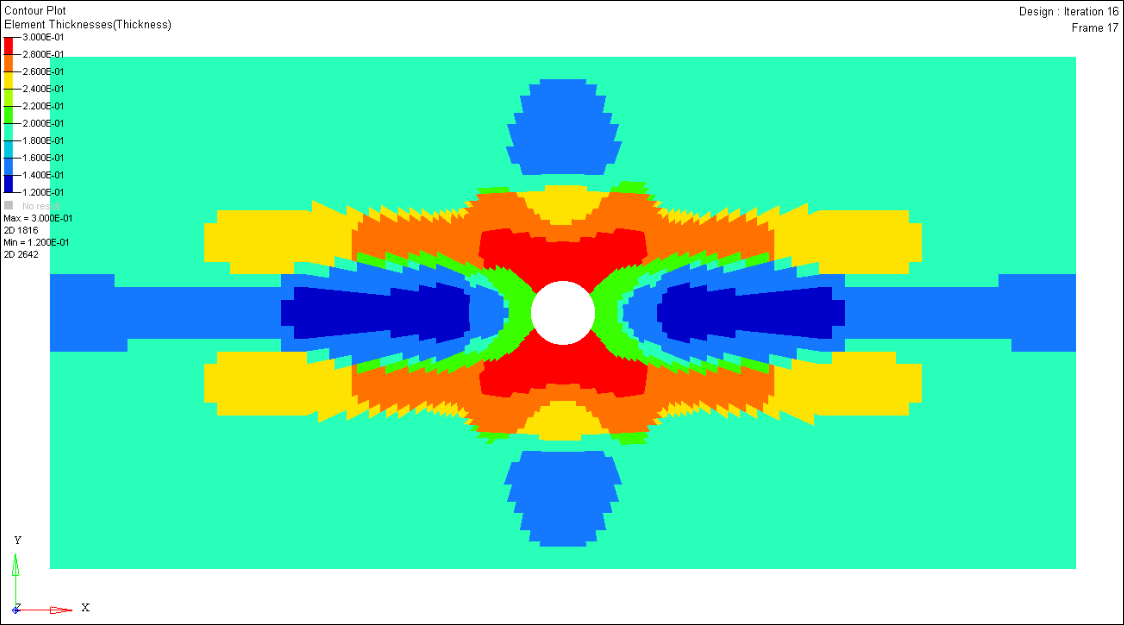
Figure 22: Element thickness contour plot (final iteration) after phase-2 size optimization
This brings us to the third and final phase of the design process in which you try to identify a proposal for the optimal stacking sequence of the plies.
Phase 3 – Ply Stacking Sequence Optimization
This algorithm is aimed at providing a global view of what the optimal stacking sequence could be. An input deck for the ply stacking sequence optimization, oht_opti_ph2_shuffling.*.fem, was generated from a previous design stage. Each ply bundle is divided into multiple PLYs whose thickness is equal to the manufacturable thickness (0.01 in this case), and the STACK card is updated accordingly. In this design phase, composite plies are shuffled to determine the optimal stacking sequence.
It is important that design performances are preserved. Hence, the optimization problem is retained as previously formulated in the size optimization phase. Two manufacturing constraints are applied:
| • | The maximum successive number of plies of a particular orientation does not exceed 4 plies. |
| • | The outermost four layers of the layup must be -45, 0, 45, 90. |
Step 1: Load the OptiStruct user profile and import the model into a new session
Follow Step 1 from the free-size phase to load the oht_opti_ph2_shuffling.*.fem file into a new HyperMesh session.
Step 2: Save the model as oht_opti_ph3.hm
Step 3: Update the design variable to input the constraints for the shuffling optimization
| 1. | In the optimization panel, click on composite shuffle to enter the composite shuffling panel. |
| 2. | Click review and select free-size to review the design variable. |
| 3. | In the parameters subpanel, click edit to enter the DSHUFFLE card. |
| 4. | Check MAXSUCC and set MSUCC to 4. |
| 5. | Check COVER and set NUMBER_OF_VANG to 4. |
| 6. | In the DSHUFFLE card editor, set VREP to 1, VANG(1) to -45, VANG(2) to 0, VANG(3) to 45, and VANG(4) to 90. |
This sets the outermost layer of the shuffling sequence to maintain one repetition of a set of -45, 0, 45, 90 degree plies. This ply set is applied to both faces of this optimization, since the laminate is symmetric.
| 7. | Click return to exit the editor and click update to update the design variable. |
| 8. | Click return to return to the optimization page. |
Step 4: Submit the shuffling job
| 1. | In the OptiStruct panel on the Analysis page, click OptiStruct. |
The following result files are generated:
oht_opti_ph3.prop
|
A property file contains the composite materials and ply properties at the last iteration.
|
oht_opti_ph3.shuf.html
|
An html file contains the history of the shuffling optimization and the view of the ply stacking sequence.
|
Step 5: Post-process the results
| 1. | Go to the directory where oht_opti_ph3.shuf.html is located and double-click the file. |
It is automatically loaded in your default Internet browser window.
The plies are color coded based on their fiber orientations.
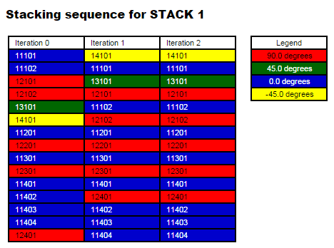
Figure 23: Shuffling Optimization History
The above image shows the history of the shuffling optimization. The columns represent the global trend of the ply stacking sequence at a particular iteration, with the last column being the final solution.
The weight of the part has not been changed during the shuffling design phase, rather the plies were reordered to obtain the maximum performance.
This light weight design therefore meets all of the performance requirements, is feasible and manufacturable.
Post-Optimization Final Analysis
The following set of steps provides a final optimized structure for comparison with the initial model.
Step 1: Load the OptiStruct user profile and open the model into HyperMesh
| 1. | Launch a new session of HyperMesh. |
| 2. | Select OptiStruct in the User Profiles dialog and click OK. This loads the user profile. It includes the appropriate template, macro menu, and import reader, paring down the functionality of HyperMesh to what is relevant for generating models OptiStruct. |
User Profiles can also be accessed from the Preferences menu on the toolbar.
| 3. | Click the Import Solver Deck icon and select oht_opti_ph3.fem. |
| 4. | Click Import. The oht_opti_ph3.fem database is loaded into the current HyperMesh session. |
Step 2: Import the final optimization properties over the existing model
| 1. | In the Import tab, browse for the oht_opti_ph3.prop file. |
| 2. | Expand the Import options section by using the drop-down toggle  . . |
| 3. | Check the box for FE overwrite and click Import to update the properties of the model with the optimized parameters. |
Step 3: Alter the control cards
| 1. | Expand the Card tree in the Model browser and right-click on the OMIT card to select Delete. |
| 2. | HyperMesh asks you to confirm the delete: Click Yes to continue. |
| 3. | Click on the OUTPUT card to load it into the Entity Editor. Change the number_of_outputs to 2 to delete the final section in the card. |
Step 4: Delete the optimization entities
| 1. | Right-click in the Model browser on the Design Variable tree and select Delete. |
| 3. | Similarly, right-click in the Model browser on the Optimization Response tree and select Delete. |
Step 5: Review the model
| 1. | Find the element visualization button and change the mode to 2D detailed element representation using the drop-down selector. |
This will thicken all shells in the model to their total thickness, displaying them as 3-dimensional representations of their thicknesses.
| 2. | Click Layers to select Composite Layers. |
This will separate the view into individual plies.
| 3. | To assist in determine which plies are which in the layup, change the element color mode to By Prop . |
This represents each of the plies in the model according to the color of its ply as shown in the Model browser. If all of the plies in the model are the same color, change the ply colors in the Model browser so that each is different to help differentiate the plies in the graphics area.
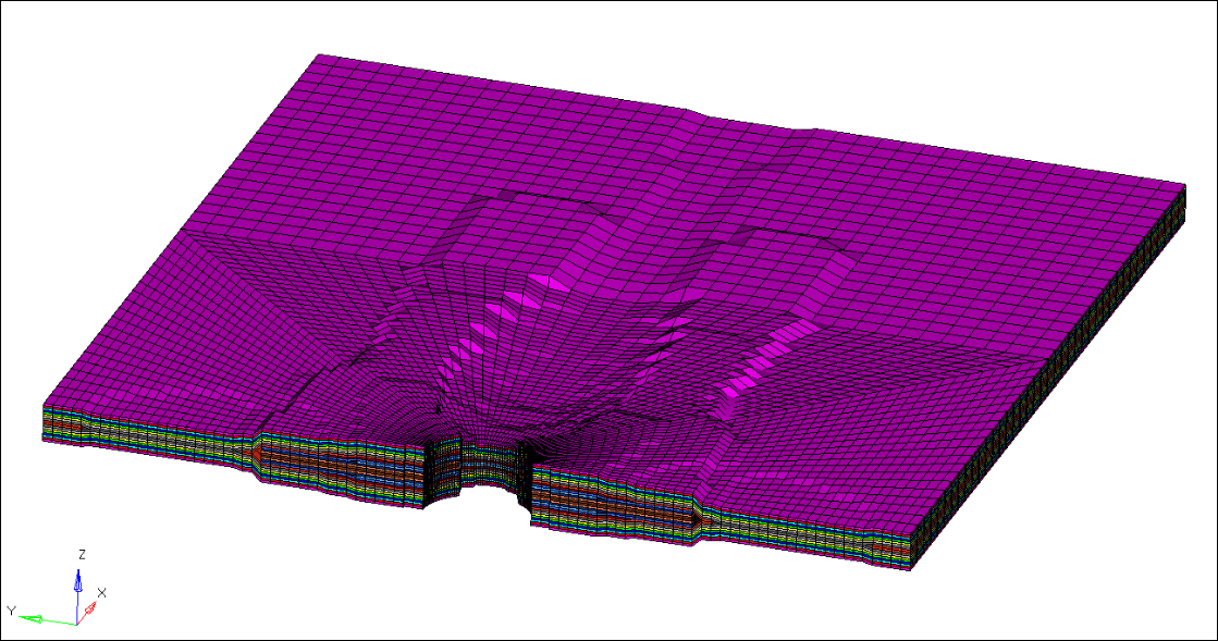
Figure 24: Visualization of model thickness in HyperMesh with half of the elements in the model masked
Step 6: Run the final analysis
| 1. | Enter the OptiStruct panel on the Analysis page. |
| 2. | Ensure that export options is set to all and run options is set to analysis. |
| 3. | Click OptiStruct to export the model and run the baseline analysis as oht_final.fem. |
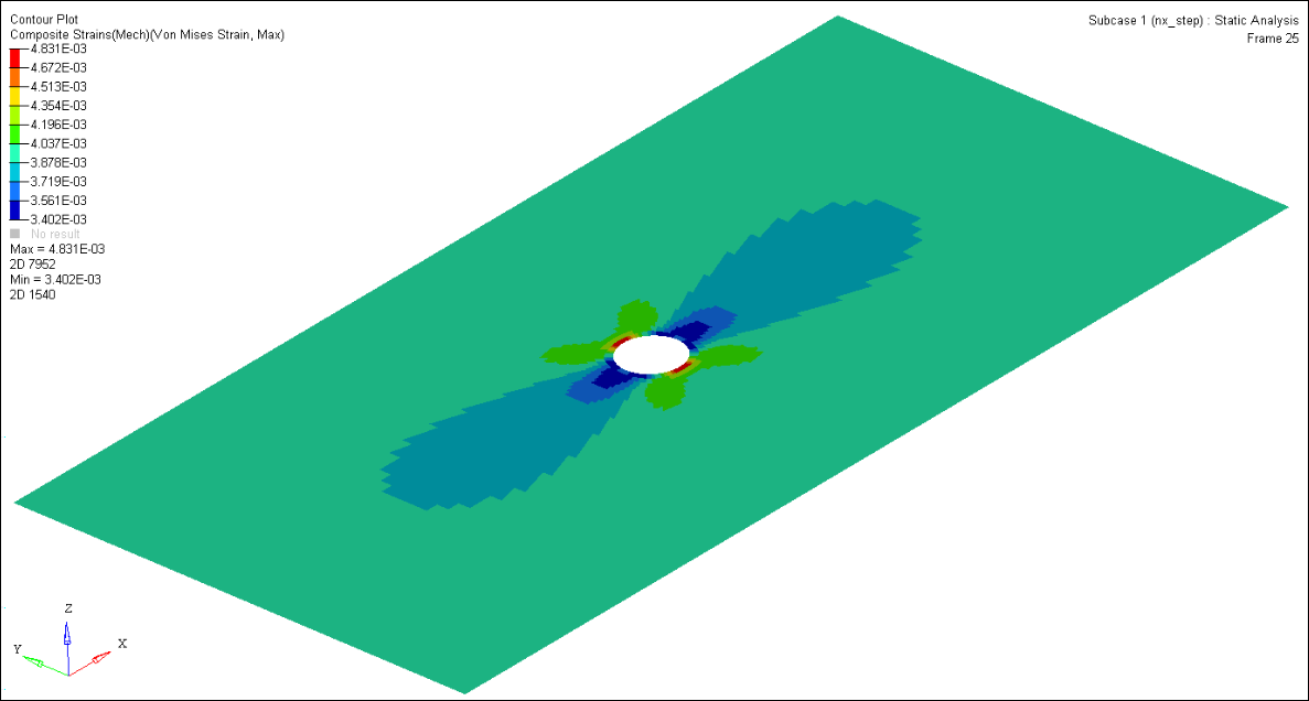
Step 7: Post-process the final analysis in HyperView
| 1. | When the run is complete, click on the HyperView button in the OptiStruct panel to load the results into HyperView. |
| 2. | Enter the Contour panel . Set Result type to Composites Strains(Mech) (s) and set the subtype to Normal X Strain. |
This corresponds to the fiber strain in the model.
| 3. | To view the individual strain contributions from any one ply, select the appropriate ply name in the Layers drop-down. Confirm that no ply exceeds 9000 microstrain (9e-3). |
| 4. | Set Result type to Composites Strains(Mech) (s) and set the subtype to Normal Y Strain. This corresponds to the matrix strain value. |
| 5. | To view the individual strain contributions from any one ply, select the appropriate ply name in the Layers: drop-down. Confirm that no ply exceeds 7000 microstrain (9e-3) for the matrix. |
The final design weighs ~0.33 lbs.
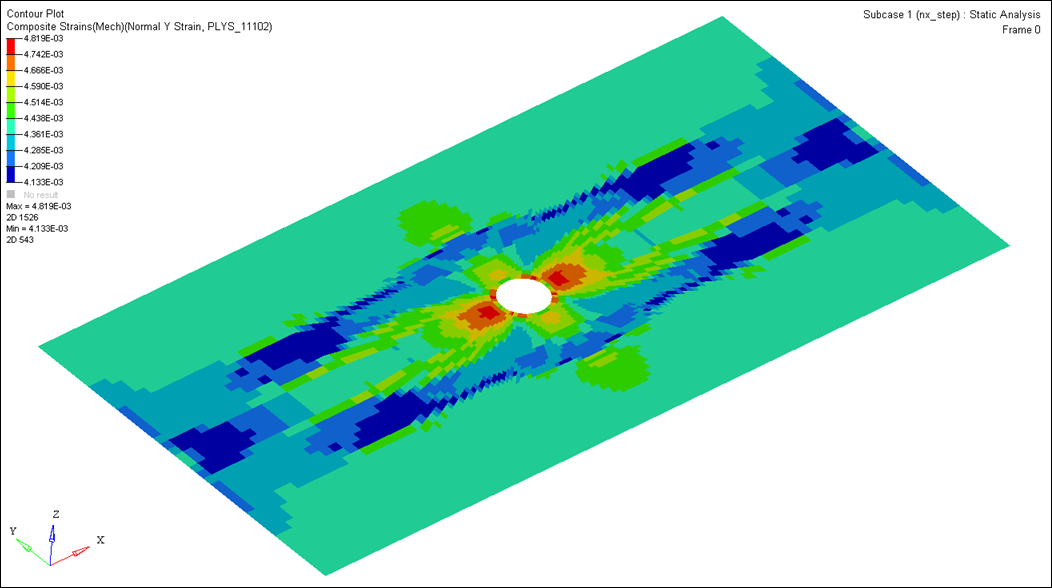
Figure 25: A plot of maximum Normal Y strain across all plies, showing that no element exceeds 0.007 me
See Also:
OptiStruct Tutorials


