OS-1040: 3D Buckling Analysis using OptiStruct

All of the files referenced in the OptiStruct tutorials are available from the website. Refer to Accessing the Model Files.

Overview

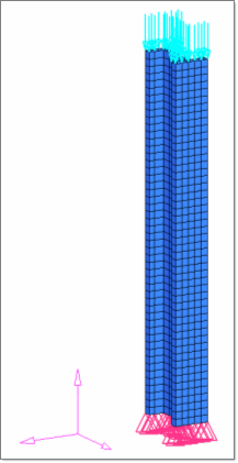
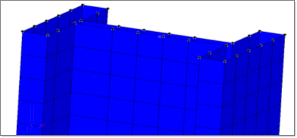
In this tutorial the steps required to perform a buckling analysis using OptiStruct are covered. The figure below illustrates the structural model used for this tutorial.

1040_model

Structural model with static loads and constraints applied.

This tutorial uses the following exercises to set up the structural model for a buckling analysis:

•	Create boundary conditions for buckling analysis

•	Post-process results

Exercise

Step 1: Launch HyperMesh, set the OptiStruct User Profile and retrieve the file

1.	Launch HyperMesh. The User Profiles dialog appears.

2.	Select OptiStruct and click OK. This loads the user profile. It includes the appropriate template, macro menu, and import reader, paring down the functionality of HyperMesh to what is relevant for generating models for OptiStruct.

3.	Click File > Open > Model. An Open Model browser window opens.

Note:

If HyperMesh Desktop was launched, use: File > Open > Model.

4.	Select the buckling.hm file you saved to your working directory from the optistruct.zip file. Refer to Accessing the Model Files.

5.	Click Open.

The structural model has already been set up to contain the necessary elements, parts, property, and material data.

Step 2: Create load collectors

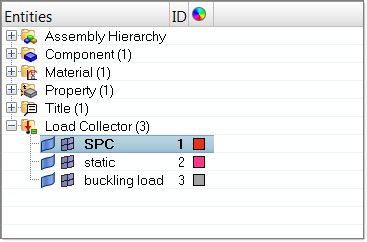
Create three load collectors (SPC, Static load and Buckling load) and assign each a color of your choice. Follow these steps for each load collector.

1.	In the Model browser, right-click and select Create > Load Collector. A default load collector template displays in the Entity Editor.

2.	For Name, enter SPC.

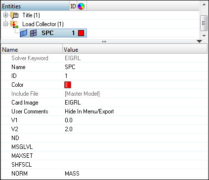
3.	Click Color and select a color from the color palette. A new load collector, SPC, is created, as shown below.

OS_1040_01

4.	Create another load collector named Static load using steps 2.1 to 2.3.

5.	Create another load collector named Buckling load.

6.	For Card Image, select EIGRL from the drop-down menu.

7.	For V1, enter the value 0.0.

8.	For ND, enter the value 2. This tells OptiStruct that you would like to extract the first two buckling modes.

Step 3: Create loads and boundary conditions for the model

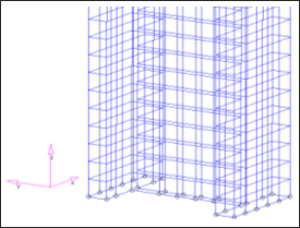
For the nodes in the following figure that show where constraints have to be created, creating these constraints and assigning them to the spc load collector is outlined in the following steps.

1.	In the Model browser, expand the Load Collector folder and right-click SPC > Make Current.

rd_loadcollector_panel_11

2.	Click BCs > Create > Constraints to open the Constraints panel.

Select all of the nodes on the bottom face of the beam, as shown in the figure (Use the nodes: on Plane option by clicking nodes >> on plane. Now, make sure that the N1N2N3B selection entities are displayed and N1 is active. Click on any three nodes on the plane shown in the figure below and click select entities. This selects all the nodes on the plane).

104_nodes_const

4.	Deselect the degrees of freedom dof4 through dof6.

5.	Click create to create the necessary boundary constraints.

6.	Click return.

7.	From the Model browser, right-click Static-load > Make Current.

8.	Click BCs > Create > Forces to open the Forces panel.

9.	Select all of the nodes on the top face of the beam, as indicated in the figure below (Use the procedure outlined in Step 3.3).

1040_nodes_static

Nodes selected for application of static forces.

10.	Set magnitude= to -10000.

11.	Set the direction selector to z-axis.

12.	Click create. The forces display in the graphics area.

13.	Click return.

Step 4: Create an OptiStruct Loadstep (also sometimes called subcase)

The last step in establishing boundary conditions is the creation of a subcase.

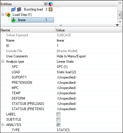
1.	In the Model browser, right-click and select Create > Load Step. A default load step template is now displayed in the Entity Editor below the Model browser.

2.	For Name, enter Linear.

3.	Click on the drop-down menu for Analysis type and select Linear Static.

4.	For SPC, click Unspecified > Loadcol.

5.	In the Select Loadcol dialog, select SPC and click OK.

6.	For LOAD, click Unspecified > Loadcol.

7.	In the Select Loadcol dialog, select Static load and click OK.

OS_1040_02

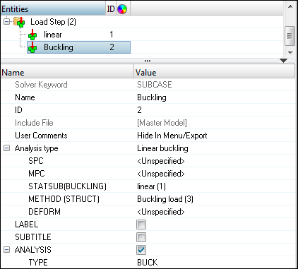
8.	Create another load step named Buckling.

9.	Click on the drop-down menu for Analysis type and select Linear buckling.

10.	For METHOD(STRUCT), click Unspecified > Loadcol.

11.	In the Select Loadcol dialog, select Buckling load and click OK.

12.	For STATSUB(BUCKLING), click Unspecified > Loadcol.

13.	In the Select Loadcol dialog, select Linear and click OK.

Note:

A STATSUB card allows for the selection of a linear static subcase for buckling analysis.

OS_1040_03

Step 5: Run both linear and buckling analysis

1.	From the Analysis page, click OptiStruct.

2.	Click save as. A Save As browser window opens.

3.	Select the directory where you would like to write the OptiStruct model file and name your input file (buckling.fem, for example) and click Save.

4.	Set the export options: toggle to all.

5.	Set the run options: toggle to analysis.

6.	Set the memory options: toggle to memory default.

7.	Click OptiStruct to launch your job. This launches the OptiStruct job.

If the job is successful, you should see new results files in the directory where HyperMesh was invoked. The buckling.out file is a good place to look for error messages that will help you debug your input deck if any errors are present.

The default files that are written to your directory are:

buckling.h3d	HyperView binary results file.
buckling.res	Results file which contains everything from displacement to stress results that can be viewed in the Post page within HyperMesh.
buckling.out	ASCII based output file of the model check run before the simulation begins and gives some basic information on the results of the run.
buckling.stat	Detailed breakdown on the CPU time used for each significant stage in the analysis.

Post process the results in HyperView

OptiStruct gives you contour information for all of the loadsteps that were run. This section describes the process for viewing those results in HyperView.

Step 6: View results of Linear Loadstep: Von Mises contour stress

1.	From the OptiStruct panel, click the HyperView icon. HyperView launches with the buckling.h3d file which contains the model and the results.

2.	Use the drop-down Subcase selector to change the analysis that you are reviewing in the current window.

1040_subcase_analysis

3.	Select Subcase 1 – Linear, in the Results browser.

4.	Click the Contour icon .

5.	Select Element Stresses (2D and 3D) as the Result type and set the sub type to von Mises.

6.	Click Apply. This should show the contour of von Mises stress.

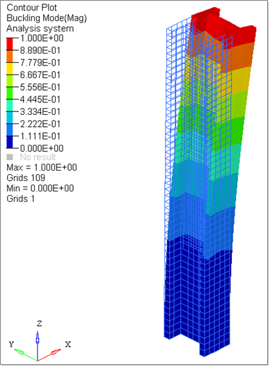
Step 7: View results of Buckling Loadstep: Deformed shape and Animating Results

1.	Click Clear Contour from the Result display control panel.

2.	Activate Subcase 2 – Buckling in the Results browser and make sure the simulation is for Mode 1.

3.	Click the Deformed panel toolbar .

4.	Under Deformed shape:, enter a Value of 10.

5.	Under Undeformed shape:, for Show:, select Wireframe from the drop-down list.

rd1040_wireframe_11A

6.	Click the Start/Pause Animation icon to view the animation.

Similarly, check the results for the 2nd mode.