The following information is common to all superelement generation methods and details the initial partitioning step involved in generating the reduced matrices. Static Condensation/Reduction is one exception, wherein, the eigenvalue problem shown in this section is not solved.
For the purpose of deriving the reduced matrices, the displacement vector u may be partitioned into displacements of inner, uo and outer, ua interface/attachment degrees of freedom.

|
(1)
|
Here, the subscript o denotes the inner degrees of freedom, and the a denotes the interface degrees of freedom (for example, ASET entry).
The static equilibrium is given as:
|
(2)
|
Where, K is the stiffness matrix and f is the force vector with the corresponding subscripts depicting the partitioning based on the inner/interface degrees of freedom.
For CBN and GM methods, an eigenvalue analysis is also performed to generate the eigenmodes.
The eigenvalue problem for a normal modes analysis of the body using a diagonal mass matrix, M is illustrated as:
|
(3)
|
Where, A are the partitioned eigenvectors of the system. Only eigenvectors pertaining to the non-attachment degrees of freedom, Ao, are used in the subsequent generation of the combined modal matrix (see CBN and GM methods below).
Static Condensation (PARAM, EXTOUT or CMSMETH (GUYAN))
The first line of equation (2) reads as:
The displacements of the inner degrees of freedom, therefore are:
|
(4)
|
 solving for
Also from equation (2):
Substituting equation (4) into this:
or
This is interpreted as:
So the reduced stiffness is:
And the reduced loading is:

The reduced matrix can now also be written based on the displacement matrix, S:
Then, using a similar transformation, you can obtain the reduced mass matrix:

The solution of the reduced linear static problem provides an exact solution, whereas the solution of the reduced eigenvalue problem, , only provides approximations to the solution of the full eigenvalue problem as only vectors that satisfy the constraint
  will be included in the solution. This can be explained by illustrating that the displacement matrix, S only consists of static displacement modes (represented by As ). The eigenmodes (represented by
  ) are not calculated in Static Condensation, therefore the reduced mass matrix is approximate.
Compliance results for reduced models
If external forces are applied to the degrees of freedom that are reduced out of the model, then the strain energy or compliance values for the complete model will not match the strain energy or compliance values for the reduced model.
From the previous section, the reduced loading is written as:
Therefore, strain energy for the reduced model is:
The strain energy for the complete model is:

Comparing the two equations, you can see that the compliance for the reduced model is missing the term,  .
.
When no external forces are applied to the degrees of freedom that are reduced out of the model, then fo is equal to zero, and the strain energy or compliance values for the reduced model match the complete model.
Dynamic Condensation (CMSMETH (CBN/GM))
Dynamic Condensation consists of both static modes and eigenmodes.
The interface or boundary degrees of freedom that are used in the construction of mode shapes should be representative of the set of force-bearing degrees of freedom in the subsequent analysis. For a finite element analysis, this refers to those nodes that connect to either the residual structure or other super element assemblies.
Supported bulk data entry for interface degrees of freedom are: ASET/ASET1, BSET/BSET1, CSET/CSET1, BNDFIX/BNDFIX1, and BNDFREE/BNDFRE1. These bulk data entries define the interface dofs to be constrained or freed.
The purpose of specifying the interface or boundary degrees of freedom for CMS is mainly to account for the static deformation due to constraint or applied forces acting on the interface degrees of freedom. A large number of eigenmodes is required, if these static modes are omitted. The flexible deformations due to constraint forces, compared to the deformation due to the body inertia forces, are often dominant in most constrained models. The inclusion of all force-bearing degrees of freedom as interface degrees of freedom is therefore an essential step to get accurate results from subsequent analyses.
The METHOD field can be set to CBN or GM on the CMSMETH bulk data entry for activation.
Craig Bampton Nodal Method (CBN)
Normal modes analysis of the fixed-interface system yields the diagonal matrix of eigenvalues,  and the matrix of eigenmodes,
  . In the normal mode analysis, you can select the cut-off frequency or the number of modes to be solved. This determines the column dimension of
  .
.
In addition, a static analysis is performed to generate the static modes. With constrained interface degrees of freedom, a unit displacement in each interface degree of freedom is applied while all other interface degrees of freedom are fixed. With unconstrained (freed) interface degrees of freedom, the inertia relief will be performed by applying a unit force in each interface degree of freedom. This yields the static displacement modes/matrix As and the interface forces, fa .
Reduced modal stiffness, Kreduced , and mass, Mreduced , matrices are now generated as follows:
The displacement matrix is written as:
Which yields,
General Method (GM)
This method also requires both static modes and the Eigenmodes, similar to CBN. However, GM includes an additional orthonormalization process to produce the diagonal reduced matrices.
From the CBN method you can see that the reduced matrices are:

An additional eigenvalue analysis is performed on the reduced matrices, as follows:
Where,  are the new eigenvalues and AGM are the eigenvectors of the system using the reduced matrices. The second reduction generates the following matrices:
Where, I is the identify matrix.
The orthogonal modes (effective modes) can be calculated, as follows:
The orthogonal modes can be directly applied on the original stiffness and mass matrices to generate the reduced GM matrices. These modes are orthogonal with respect to the original stiffness and mass matrices.
Generating the Matrices
Through the inclusion of certain Bulk Data and I/O Options entries described here, static and dynamic reduction may be performed on a structure and the reduced matrices written to a file for use in subsequent analyses.
PARAM,EXTOUT controls the file format to which the reduced matrices are written (either .pch, .dmg, .op2, and .op4). With CMSMETH, the reduced matrices are output in an .h3d file, unless OUTPUT,H3D,NONE is defined. The I/O option entry DMIGNAME provides you with control of the name of the matrices written to the .pch and .dmg files. This is an optional entry and if not used, matrices are given the suffix “AX.”
Static reduction can be performed in two ways. One is to specify ASET/ASET1 with PARAM,EXTOUT (no CMSMETH). The other way is to specify ASET/ASET1 and CMSMETH (METHOD field=GUYAN) with or without PARAM,EXTOUT.
For the static reduction without CMSMETH, if the SUBCASE is for static analysis, by default the reduced mass matrix will not be created. However, PARAM,MASSDMIG,YES can be used to create the reduces mass matrix for static analysis. For eigenvalue analysis, the mass and stiffness matrix will be reduced, but there is no reduced load vector. Note that the static reduction is not recommended for dynamic analysis, because the mass is not as accurate as dynamic reduction.
For dynamic reduction, stiffness, mass, static loading, structural and viscous damping, and fluid-structure coupling matrices can all be generated.
Dynamic reduction is activated by the presence of the I/O Option CMSMETH. The I/O Option references a CMSMETH Bulk Data entry, which defines the method of matrix reduction to be used (CBN or GM methods apply to dynamic reduction). When CBN or GM is the selected method, the frequency range or number of modes to be calculated and the starting SPOINT ID for storing the modal data are also defined on CMSMETH. For GUYAN, this additional information is ignored.
The export of the model to an .h3d file can be controlled using the MODEL output statement. This allows for only a small portion of the model or a “display model” (a coarse representation of the structure consisting of PLOTELs) to be exported.
For dynamic reduction super elements written to the .h3d file, there is no interior grid or element data stored by default. However, the MODEL data can be used to specify interior grids for displacement, velocity, or acceleration results, and interior elements for stress and strain results in the residual run. The SEINTPNT data can be used to convert the interior points to exterior points in the residual run, so that they can be used as connection points, loading points, or response points in optimization.
Using the Matrices in a Finite Element Analysis
To use the reduced matrices that were written to an .h3d file, the ASSIGN I/O option must be used to assign names to such matrices. The reduced matrices stored in .pch or .dmg formats can be included in residual run with INCLUDE bulk entry. Unlike matrices stored in .pch or .dmg formats, those stored in the .h3d file are named on retrieval, rather than on creation. The ASSIGN, H3DDMIG command provides a suffix “matrixname” for the matrices retrieved from that file. Once matrices in an .h3d file have been assigned a name, they may be referenced using one of the subcase information entries listed below. All of the matrices in the .h3d file are used in the analysis by default. If only some of the matrices are to be used, then use the K2GG, M2GG, K42GG, and B2GG data to specify which matrices are to be used. The unreferenced matrices will not be used in this case.
Reduced matrices that are written to .pch files are stored as DMIG bulk data input. As these reduced matrices are already in a recognized input format, the files simply need to be included in the bulk data section by an INCLUDE statement.
Reduced matrices that are written to a .dmg file are stored in a binary format. Similar to the .pch file, these reduced matrices simply need to be included in the bulk data section by an INCLUDE statement.
As matrices are referred to by name, it is important to ensure that when multiple reduced matrices are used that they have unique names. Matrices may be chosen through one of the following subcase information entries as either stiffness, mass, damping, or load matrices.
The SEINTPNT can be used to convert the interior points specified by the MODEL data in the creation run to exterior points in the residual run, so that they can be used as connection points, loading points, or response points in optimization.
The K2GG subcase information entry references a matrix by name, indicating that it is a stiffness matrix. The stiffness matrix must be symmetric and it applies to all subcases.
The M2GG subcase information entry references a matrix by name, indicating that it is a mass matrix. The mass matrix must be symmetric and it applies to all subcases. Gravity and centrifugal loads will be generated from the external mass matrix (M2GG) in residual run by default (can be adjusted by PARAM,CMSALOAD). Gravity and centrifugal loads can also be generated in DMIG run as the reduced loads (P2G). The caution needs to be made to make sure no doubling effect of Gravity/Centrifugal loading with M2GG and also from P2G.
The B2GG subcase information entry references a matrix by name, indicating that it is a viscous damping matrix. The viscous damping matrix must be symmetric and terms are added to it before any constraints are applied.
The K42GG subcase information entry references a matrix by name, indicating that it is a structural element damping matrix. The structural element damping matrix must be symmetric and terms are added to it before any constraints are applied. This can only be generated from material GE specified on material card.
The P2G and P2GSUB subcase information entries reference a matrix by name, indicating that it is a load matrix. The load matrix must be columnar and terms are added to it before any constraints are applied. Gravity and centrifugal loads are not considered on the external mass matrix (M2GG). Gravity and centrifugal loads must be included in generating the reduced loads. The P2G and P2GSUB can then be used in DMIG input to get the exact static results. P2G must be used above the first SUBCASE. If there are multiple load vectors in the DMIG, then they will be applied in successive static SUBCASE until they are all used or until every static SUBCASE has a load vector. P2GSUB is used within a specific SUBCASE. If there is more than one load vector in the DMIG, then P2GSUB can be used to specify which load vector is to be used in that SUBCASE.
The A2GG subcase information entry references a matrix by name, indicating that it is a fluid-structure coupling matrix. Only one instance of the fluid-structure coupling matrix is allowed.
Example 1 (Static Condensation)
Figure 1 shows a finite element model composed of two components: a design component and a non-design component. The structure is fully clamped along the left-hand edge and has a downward vertical force applied along its right-hand edge. This example will demonstrate how to replace the non-design component with a set of reduced matrices at the interface nodes (the nodes which are common to both components) for both an analysis problem and an optimization problem.
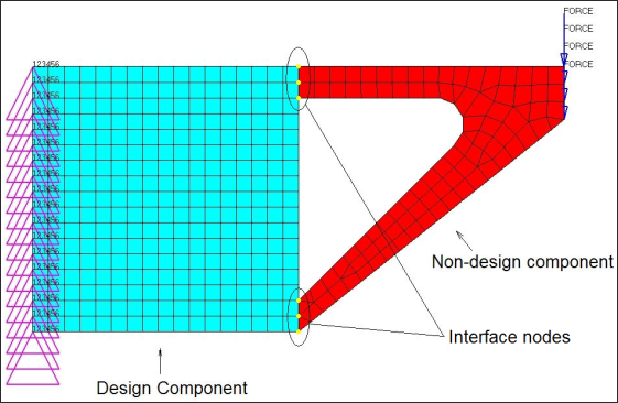
Figure 1: Example model indicating design and non-design components and boundary nodes.
First of all, a linear static analysis is performed on the complete structure. The displacement and von Mises stress results from this analysis (Figure 3).
Next, a reduced stiffness matrix and a load vector are generated for the non-design component. This is achieved by creating a new finite element model containing just the non-design component and the loads and boundary conditions directly applied to that component (Figure 2).
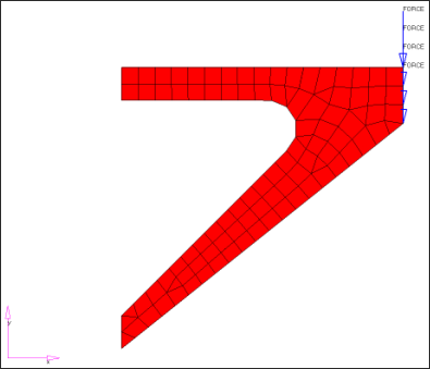
Figure 2: Reducing out the non-design component.
All of the degrees of freedom at the interface nodes (Figure 1) are selected as boundary degrees of freedom. ASET or ASET1 bulk data entries are used to indicate this. The reduced matrices output is requested through the inclusion of the PARAM, EXTOUT, DMIGPCH bulk data entry. The model is submitted to OptiStruct, resulting in the creation of the file filename_AX.pch which contains the reduced matrices in ASCII format. (Had PARAM,EXTOUT,DMIGBIN been used, the reduced matrices would be written in binary form to the file filename_AX.dmg).
The non-design component can now be replaced in the original model by its reduced matrix representation. This is done by manipulating the original model as follows:
| 1. | Delete the bulk data entries for the nodes and elements of the non-design component. |
| 2. | Delete all loads and boundary conditions that were only applied to the non-design component. |
| 3. | Include the file containing the reduced matrices in the bulk data section. |
| 4. | Select the reduced stiffness matrix with the subcase information entry K2GG. (In this example, the reduced stiffness matrix will have the default name KAAX). |
| 5. | Select the reduced load vector with the subcase information entry P2G. (In this example, the reduced load vector will have the default name PAX). |
Figure 4 shows the displacement and von Mises stress for the design component when the non-design component was replaced by a reduced matrix representation. It can clearly be seen, they match perfectly with the original model's results.
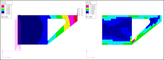
| (a) Displacements | (b) von Mises Stress |
Figure 3: Displacement and von Mises stress results for a linear static analysis on the complete structure.
| (a) Displacements | (b) von Mises Stress |
Figure 4: Displacement and von Mises stress results for a linear static analysis with reduced matrix substitution.
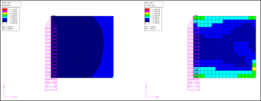
Finally, for both the complete structural model and the reduced matrix model, a topology optimization was performed. For both models, the design component was identified as designable, the objective was to minimize the global compliance, and an upper limit of 50% was put on the volume fraction. The optimization results are shown in Figure 5.
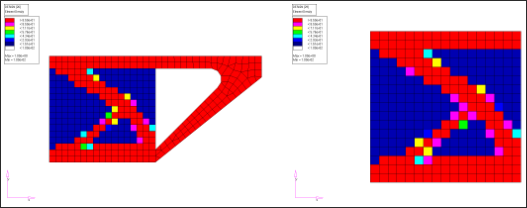
| (a) Complete Structure | (b) Reduced Matrix Substitution |
Figure 5: Density results for a topology optimization.
Example 2 (Static Condensation vs CBN)
Figure 6 shows a finite element model running Normal Modes Analysis to compare the accuracy of static condensation and the dynamic condensation using CBN. The results are compared against the full model results.
The comparison clearly indicates that the dynamic reduction with CBN is highly accurate for this type of analysis, when compared to Static Condensation since the mass matrix is reduced accurately.
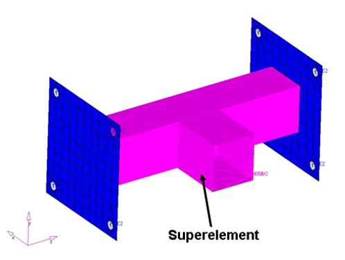
Figure 6: Normal Mode Analysis model.
Eigenmodes
|
Full
Model
|
Static
Reduction
|
Dynamic Reduction
(CMSMETH, CBN)
|
1
|
110.67
|
444.66
|
110.67
|
2
|
167.00
|
765.31
|
167.00
|
3
|
352.39
|
769.06
|
352.39
|
4
|
1272.95
|
2547.13
|
1272.96
|
5
|
1614.57
|
2923.56
|
1632.78
|
See Also:
Introduction: Superelements in FEA (DMIG)


