Coupling

Coupling refers to the forces and moments generated in a bushing to oppose the overall deformation of the bushing. These forces and moments are independent of any coordinate system that might be used to measure the deformation or deformation velocity. Coupling is an important factor when the bushing characteristics are non-linear.

Below we provide information on the formulation for coupling followed by three examples that show how coupling affects bushing force and torque output:

The Altair Bushing Model supports three options for coupling:

•	Cylindrical coupling (2-dimensional).

•	Spherical coupling (3-dimensional).

•	No coupling.

Two-dimensional coupling and three-dimensional coupling are analogous, and therefore, this guide explains coupling in terms of the two-dimensional concept.

For cylindrical coupling, assume:

•	A bushing has been fitted in two radial directions: x and y.

•	The internal states for the bushing are d, the bushing deformation, v, the bushing velocity, and q. These can change with direction.

•	Gx (d,v,q) defines the force function in the x-direction, as obtained by the fitting process.

•	Gy (d,v,q) defines the force function in the y-direction, as obtained by the fitting process.

•	During simulation, at any time t, the bushing undergoes deformations of (x, y) and deformation velocities of .

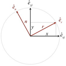
The diagram below shows the deformations and force vectors in the bushing. The J Marker is used as the coordinate system for all calculations.

coupling

	are the unit vectors along the x- and y-axes of the J marker. For cylindrical coupling, axial deformation is uncoupled. Only the x- and y-forces are coupled.
	is a unit vector along the deformation vector.
r	is the magnitude of the deformation. Its components along are denoted as x and y respectively.
	is a unit vector orthogonal to the deformation vector. It points to the tangential velocity that may exist in the bushing.

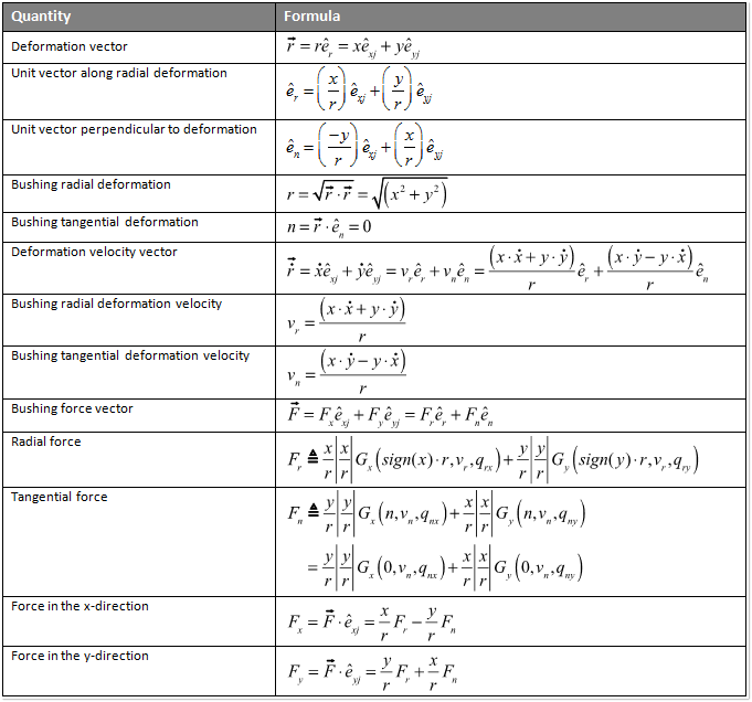
The table below shows the various quantities of interest and how they are calculated:

coupling2

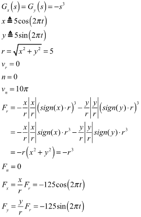
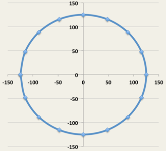
Example 1: Isotropic Bushing with No Damping and Constant Rotating Deflection

A constant deflection of 5 units stretching the bushing and rotating at 2*π radians/sec is imposed on the bushing. Rotation occurs in the X-Y plane of the J-Marker.

The following equations show the forces Fx and Fy computed by the coupling formulation. The plot shows that Fy vs. Fx is a circle as expected.

eq_coupling4

Fy vs. Fx

eq_coupling3

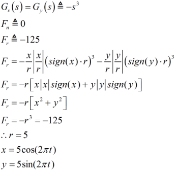
Example 2: Isotropic Bushing with No Damping and Constant Rotating Force

A constant tensile force of 125 units, rotating at 2*π radians/sec is imposed on the bushing. The force rotates in the X-Y plane of the J-Marker.

The following equations show the deformations x and y as computed by the coupling formulation. The plot shows y vs. x is a circle as expected.

eq_couplin6_first_half

eq_couplin6

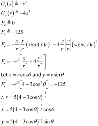
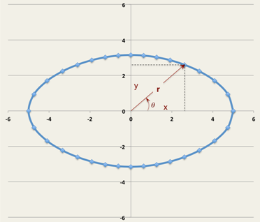
Example 3: Anisotropic Bushing with No Damping and Constant Rotating Force

A constant tensile force of 125 units, rotating at 2*π radians/sec, is imposed on the bushing. Rotation occurs in the X-Y plane of the J-Marker.

The following equations show the deformations of x and y as computed by the coupling formulation. The plot shows that since the bushing is non-isotropic, the y vs. x plot is not a circle, but a smooth, elliptical, closed-curve as expected.

eq_coupling8_first_half

y vs. x

eq_coupling8