This section describes the fitting process and the main challenges associated with it for a nonlinear, dynamic system.
Identification Problem for Fitting
The bushing identification is formulated as follows:
(Click to enlarge)
such that the constraints:

(Click to enlarge)
Subject to limits on the parameters p:
(Click to enlarge)
Understanding the Fitting Process
This section describes the three-step fitting process of the MIT. This process provides robust and accurate fitting results without user intervention.
The fitting process begins with an optimization run. The goal of this optimization is to obtain a reasonable set of starting values for the design parameters.
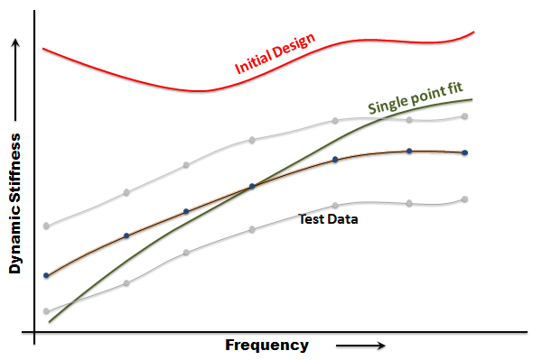
| • | The fitting tool uses the parameters defined in the Initial .gbs file, and then attempts to refine these values using a method known as single-point fitting. |
| • | The objective of single-point fitting is to select a single point in the middle of the data, and then fit the parameters to that selected point. The parameters are used to compute the cost function, Cost (b), for all frequencies and amplitudes. |
| • | If the cost is less than the cost calculated with the original design, the new design is accepted as the starting point. |
| • | If the cost is greater than the cost computed with the original design, an adjacent point is selected and the single point fitting is repeated. |
| • | This operation continues until a better initial design is found. In the unlikely scenario that no single point fit is better than the original design, the original design is used as the starting point. |
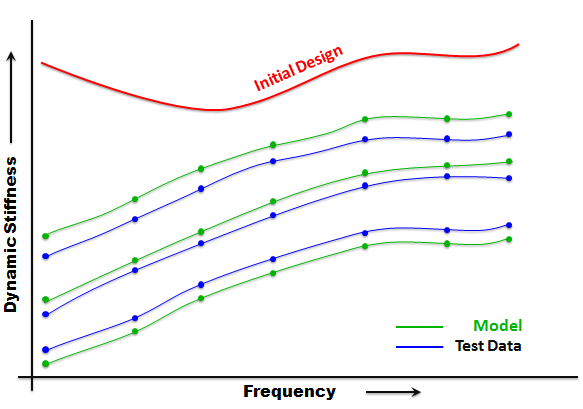
Single point fitting is very fast and the optimizer converges in just a few iterations. The following plot shows the effect of a single point fit:
|
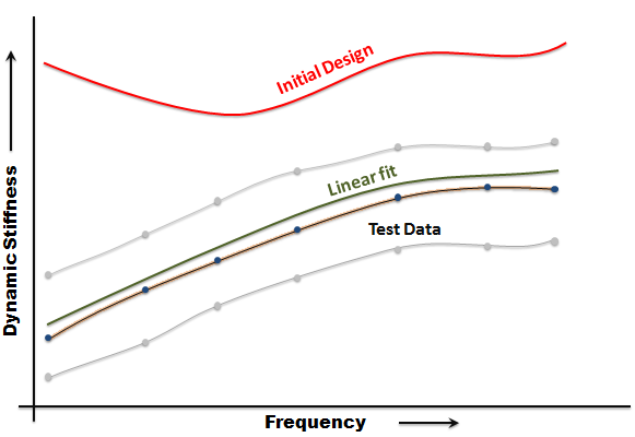
The purpose of this fitting is to determine the overall shape of the dynamic stiffness and phase angle curves.
| • | The results from Step 1. are used as the starting point. |
| • | You can observe from the plot below that the model is linear in terms of the parameters k0, k1, k2, c0, c1 and c2. Non-linearity occurs in the parameters p0, p1, p2, q0, q1 and q2. Therefore, p0, p1, p2, q0, q1 and q2 are kept fixed at reasonable values as an optimization is run to determine k0, k1, k2, c0, c1 and c2. |
| • | Since the model is linear when parameters p0 through q2 are fixed, it does not show any amplitude dependency. Moreover, the equations can be solved using linear methods. |
| • | The following plot shows the effect of a linear fit: |
|
The purpose of this step is to fit all of the data, for example, the frequencies, amplitudes and preloads, to all of the parameters in the model.
| • | The output from Step 2. is used as the starting point for yet another optimization run. |
| • | All terms in the model, linear and nonlinear, are included in the calculations. |
| • | The entire set of data, all frequencies, amplitudes and preloads, are fitted. |
| • | The optimizer returns when it has either met its goal or when it cannot further reduce the cost function. |
| • | The following plot shows the effect of a global fit: |
|
Challenges in the Fitting Process
This section discusses the three main challenges that can occur when using gradient-based approaches to fit bushing model data to test data:
Gradient-based models require a feasible initial guess. To learn how to obtain a good initial guess, see Step 1 in the previous section.
In the rare situations that you need to supply a better initial guess, you can do so using the Fit and Analyze tabs where you can specify the initial values for all of the parameters. Before attempting to change any of these values, be sure to clearly understand the concept of parameters as your choice of values directly affects your solution. To learn more about parameters, see Fit Data.
|
How do I know that the optimization has converged to an acceptable fit?
The metrics commonly used to assess convergence are:
| • | The maximum deviation between the model and experiment in the dynamic stiffness is less than 10%. |
| • | The maximum deviation between the model and experiment in the loss angle is less than 2°. |
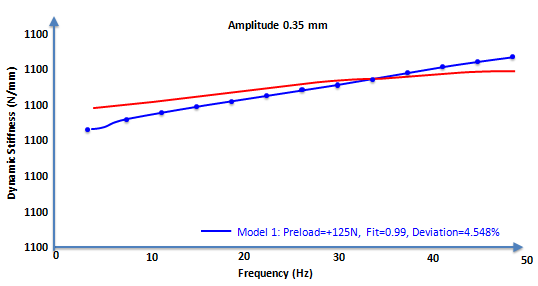
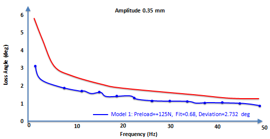
The MIT displays the maximum deviations in every plot it generates. By reviewing the plots, you can assess whether the results have converged or not. The figure below shows two plots: the one on the left shows results that meet the convergence metric; the one on the right shows where the results do not meet the metric. In both cases, the blue curve represents measured data and the red curve the model behavior. The legend indicates whether or not the convergence metric is met.
You can review the fit .log file and the output .gbs file to see the results of the optimizer. The following is an example of a fitting that works. The final fit metric is shown in green.
Fit Summary For Linear + Nonlinear Model Fitting
-----------------------------------------------
|
Cost function value
|
= 113.153
|
Max Kdyn Deviation
|
= 3.093%
|
Max Loss Angle Deviation
|
= 1.766 degrees
|
Score for k_magnitude
|
= 0.996
|
Score for loss_angle
|
= 0.927
|
The following example is from a .log file and shows where a fit metric has not been met. The metric not satisfied is shown in red.
Fit Summary For Linear + Nonlinear Model Fitting
-----------------------------------------------
|
Cost function value
|
= 188.146
|
Max Kdyn Deviation
|
= 6.320%
|
Max Loss Angle Deviation
|
= 3.358 degrees
|
Score for k_magnitude
|
= 0.991
|
Score for loss_angle
|
= 0.947
|
|
The default .opt file in the MIT has a set of defaults that has been tested successfully in over 100 physical bushing test data sets. These defaults have been found to work well, and we recommend that you do not change these without due consideration.
However, on occasion, you may find it necessary to modify the limits of the design variables. Many of these parameters are associated with a physical bushing and it is important to ensure that the limits you specify are likewise realistic for a physical bushing. For instance, a stiffness parameter may not have its lower limit set to a value less than zero.
The following table shows the lower and upper bounds for each design parameter for rubber and hydromount bushings. Lower limits that must not be decreased are shown in red.
Rubber Bushings
|
Hydromounts
|
Name
|
Lower Limit
|
Upper Limit
|
Name
|
Lower Limit
|
Upper Limit
|
K0
|
0.0
|
10000.0
|
K0
|
0.0
|
10000.0
|
K1
|
0.1
|
20000.0
|
K1
|
0.1
|
20000.0
|
K2
|
0.1
|
100.0
|
K2
|
0.1
|
100.0
|
C0
|
0.0
|
700.0
|
C0
|
0.0
|
700.0
|
C1
|
0.0
|
1000.0
|
C1
|
0.0
|
1000.0
|
C2
|
0.0
|
10.0
|
C2
|
0.0
|
10.0
|
P0
|
0.5
|
10.0
|
P0
|
0.5
|
10.0
|
P1
|
-10.0
|
10.0
|
P1
|
-10.0
|
10.0
|
P2
|
0.01
|
2.0
|
P2
|
0.001
|
2.0
|
Q0
|
0.5
|
10.0
|
Q0
|
0.5
|
10.0
|
Q1
|
-10.0
|
10.0
|
Q1
|
-10.0
|
10.0
|
Q2
|
0.01
|
2.0
|
Q2
|
0.001
|
2.0
|
R
|
0.000001
|
1000.0
|
R
|
0.001
|
10.0
|
|
|
|
MH
|
0.000001
|
10.0
|
|
|
|
KH
|
0.0
|
100000.0
|
|
|
|
CH1
|
0.0
|
1000.0
|
|
|
|
CH2
|
0.0
|
1000.0
|
|
|
|
J0
|
0.5
|
10.0
|
|
|
|
J1
|
-10.0
|
10.0
|
|
|
|
J2
|
0.01
|
2.0
|
|
|
|
L0
|
0.5
|
10.0
|
|
|
|
L1
|
-10.0
|
10.0
|
|
|
|
L2
|
0.01
|
2.0
|
Is setting the upper and lower bounds for the parameters important for a successful fit?
Setting the proper upper and lower boundaries for the parameters is very important for two reasons:
| 1. | The boundary for each of the design variables is a property particular to both the type and the direction of a bushing. |
| 2. | An improper boundary set can cause the optimizer to go into in an unfeasible region. This can cause the fitting to fail, or worse, it can create a bushing that is inherently unstable. Such a bushing is prone to cause simulation failures by adding energy into the system. |
How do I define the upper and lower bounds for the bushing parameters?
| 1. | Specify the boundary from its feasible physical range, based on the type and the direction of a bushing. Use the considerations from Fitting Challenge 1. above to obtain an initial guess. |
| 2. | Review the results produced by the optimizer, which are located in the fit .log file. You can use the MIT to review the .log file. In the following example, you can see that four of the design variables, K1, C2, K2 and R are stuck at the boundary. The four asterisks (****) at the end of the line indicate this. |
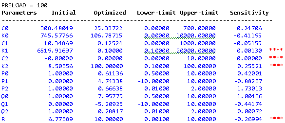
| 3. | Notice that parameters K1 and C2 are at their lowest physically meaningful values. Do not change these! |
| 4. | Parameters K2 and R are at the upper boundaries. If the optimization results are not satisfactory, you can increase the upper limit of these parameters. Changes in the limits should be gradual as the optimizer could respond to the changes rather dramatically. You should not exceed a 20%-25% change in the limits in one step. |
|
|