Bushing measurements are typically provided in the frequency domain, and not in the time domain. Thus, for a given preload and frequency, the bushing is typically subjected to a sinusoidal input at a given frequency. The bushing response at steady state, for the given preload and frequency, is measured in terms of a dynamic stiffness (Kd ) and a loss angle  .
.
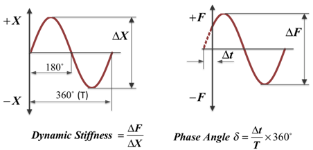
Dynamic stiffness is the frequency dependent ratio between a dynamic force and the resulting dynamic displacement. The force can have two components: a displacement-dependent or spring-force component and a velocity-dependent or damping-force component.
Loss angle is defined as the phase angle between the displacement and the force. This phase difference is caused by the presence of the damping forces. The ratio of the damping force to the spring force is often called the loss tangent. It is the tangent of the loss angle.
These quantities are described in the following figure:
Example of a Steady State Response of a Nonlinear Dynamic System
Assume that a nonlinear system is provided with a sinusoidal input at a constant frequency ω0. The system responds with a variety of harmonics as you see summarized in the following figure:
The dynamic stiffness and phase angle are the response values of the system at the first harmonic ω0.
Calculating the Dynamic Stiffness and Loss Angle of a Bushing
This section discusses how to analytically calculate dynamic stiffness and loss angle of a bushing from the bushing's equations. Examples in this section are based on a rubber bushing though you can apply the same calculation methods to hydromount bushings.
Rubber Bushing Equations
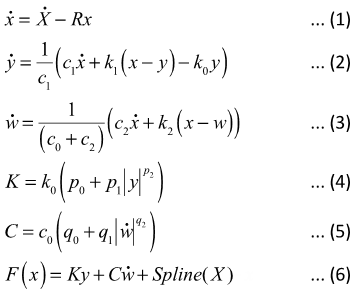
In the above equations:
| • | X is the input displacement provided to the bushing. |
| • | R is the cutoff frequency associated with a first order filter that acts on the input X. |
| • | x is the dynamic content of the bushing input X. This is the filter output. |
| • | y and w are the internal states of the bushing; ẏ and ẇ are their time derivatives. |
| • | k0 and k1 represent the bushing rubber stiffness. |
| • | k2 is used to control the stiffness at large velocities. |
| • | c0 produces the roll-off observed in the experimental data at low velocities. |
| • | c1 accounts for the relaxation of the bushing impact force. |
| • | c2 represents the viscous damping observed at large velocities. |
| • | p0, p1 and p2 are scale factors for stiffness. |
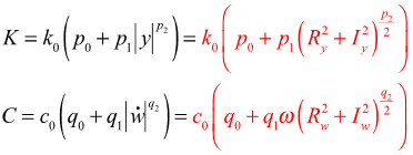
| • | K is the effective stiffness of the bushing. |
| • | q0, q1 and q2 are scale factors for damping. |
| • | C is the effective damping of the bushing. |
| • | X0 is the deformation due to preload (zero, if there is no preload). |
| • | Spline (X) is the static force response of the bushing. |
The States
For a sinusoidal input, at steady state and considering only the lowest harmonic, the inputs and states for the bushing assume the form:
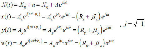
X0 is the deformation due to an initial preload  is the magnitude of the sinusoidal input and ω is its angular frequency. For each test, X0 and ω are known. The quantities Rx, Ix, Ry, Iy, Rw, Iw are not known and can be determined by the governing equations.
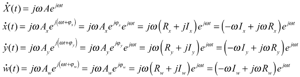
The State Derivatives
At steady state, the time derivatives of the states assume the form:
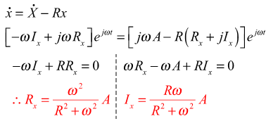
Steady State Equations for a Rubber Bushing: Equation 1
At steady state, equation (1) can be expressed:
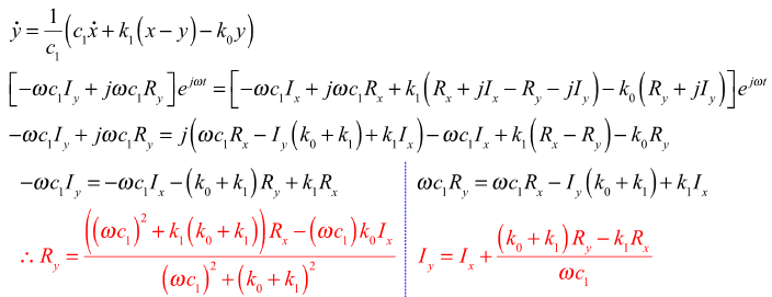
Steady State Equations for a Rubber Bushing: Equation 2
At steady state, equation (2) can be expressed:
Steady State Equations of a Rubber Bushing: Equation 3
At steady state, equation (3) can be expressed:
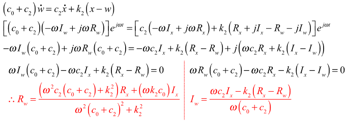
Steady State Equations of a Rubber Bushing: Equations 4 and 5
At steady state, equations 4 and 5 can be expressed:
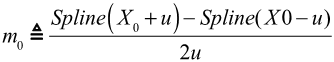
Steady State Equations of Rubber Bushing: Equation 6
In the physical test of the bushing, the bushing is provided an initial preload deformation, X0, and a dynamic oscillation, u, is superposed on top of it. Therefore at steady state, the average slope for an oscillation, u, about a preload, X0, is:
The static response of the bushing for a dynamic oscillation, u, is therefore:
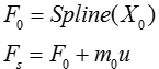
Dynamic Stiffness is the ratio of the force change per oscillation cycle divided by the displacement change. The static force F0 at the operating point cancels out during these calculations. We can equivalently achieve this by just subtracting F0 from the force, therefore:
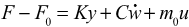
Substituting the expressions for y, ẇ, X and x, one gets:
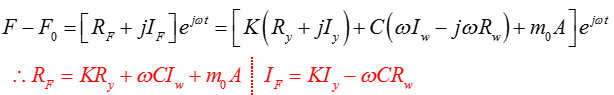
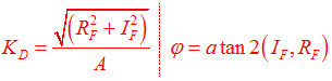
Dynamic Stiffness and Loss Angle of a Bushing
You can compute the dynamic stiffness and loss angle as: