|
»Click here to display Table of Contents«
|

View Data |

|

|

|

|
|
View Data |
|
|

|

|
|
»Click here to display Table of Contents«
|
View Data |
|
|
|
|
|
View Data |
|
|
|
|
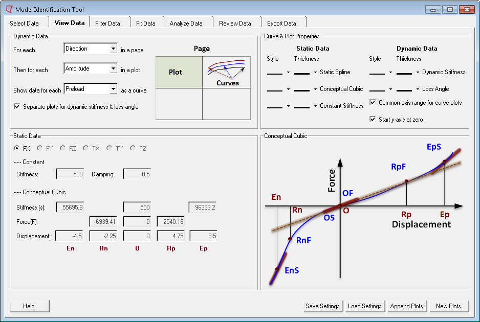
The View Data tab lets you specify, plot and view your data. The tab is divided into three working sections: Dynamic Data, Static Data, and Curve and Plot Properties. A fourth section displays a static image of the Conceptual Cubic.
| • | Select the View Data tab, and the following page appears: |
From the View Data tab, you can define the following:
This is the area of the View Data tab where you can define the display layout for dynamic stiffness and loss angle measurements. You have the option of sorting your data by Direction, Amplitude and Preload. The default setting displays all data for a direction first. For each direction, data for a specific amplitude is displayed in a plot window. In each plot window several curves are drawn—one for each preload. Each curve is the graphical representation of the dynamic stiffness (loss angle) vs. frequency relationship. You can also specify whether the dynamic stiffness and loss angle are to be plotted in the same window or in separate windows (default). You select a checkbox to indicate your preference.
|
This is the area of the View Data tab that displays the static properties derived from the experimental measurements. The tab includes three representation options for the static data.
|
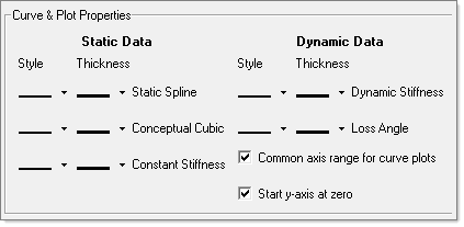
The Curve and Plot Properties options let you define the line-style and line-thickness for dynamic stiffness and loss angle curves. The default option is a line-style and coloring scheme that shows the most contrast between the curves.
|
A series of four buttons at the bottom of the View Data tab lets you do the following:
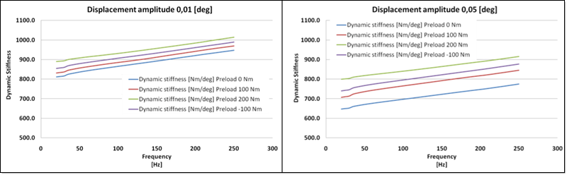
You can use the New Plots button to plot dynamic and static data as follows:Dynamic DataDynamic data is plotted according to the scheme you define in the Dynamic Data section of the View Data tab. The following sample plots show Dynamic Stiffness vs. Frequency for various amplitudes for the FX direction:
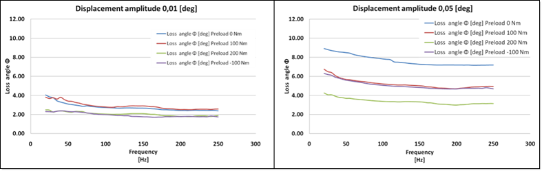
The following are sample plots for Loss Angle vs. Frequency for various amplitudes for the FX direction.
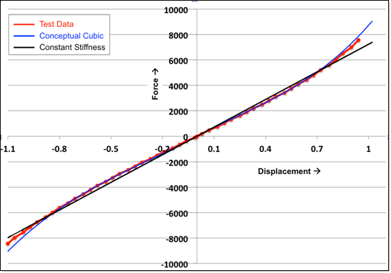
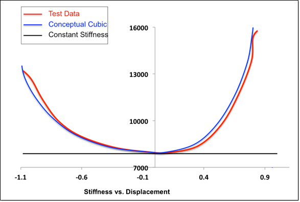
Static DataFollowing are two plots for static data. Each plot contains three curves: the red curve indicates experimental data, the blue curve indicates the conceptual cubic, synthesized from the static data, and the black curve indicates constant stiffness. The following plot shows the Force vs. Displacement behavior for the three curves:
The following plot shows the Stiffness vs. Displacement behavior of the bushing.
|