In this tutorial, you will learn how to:
| • | solve an ADM/ACF model that has flexbodies using MotionSolve. |
| • | use the Add Object panel in Hyperview and view the transient analysis results from MotionSolve. |
Theory
You can submit Adams dataset language files (ADM and ACF) directly to MotionSolve, thus avoiding manual translation. The Adams model is first automatically translated into the MotionSolve XML format and then it is solved. If the Adams model has a flexible body represented by the MNF and MTX files, the MotionView Flexprep utility will be used to generate an H3D flexible body file (using the MNF file). This H3D flexbody file is the MotionSolve equivalent of the Adams MNF and MTX files. It holds the mass and inertia properties, as well as the flexibility properties which allow the body to deform under the application of loads. The deformation is defined using a set of spatial modes and time dependent modal coordinates.
Process
In this tutorial, an Adams single cylinder engine model (ADM and ACF) is provided. To improve the accuracy of the model responses, the connecting rod is modeled as a flexbody (MNF and MTX). This chapter deals with transient analysis of this single cylinder engine model using MotionSolve.
We will modify the ACF file to include an argument that would generate a flexbody H3D file. MotionSolve internally calls OptiStruct, which generates the H3D flexbody file. The ADM and ACF is translated into MotionSolve XML format and solved. MotionSolve outputs the results H3D file, which can be loaded in HyperView for animation. In HyperView, external graphics (for piston and crank) can be added for visualization.
MotionSolve supports most of the Adams statements, commands, functions, and user subroutines. Refer to the MotionSolve User’s Guide help for additional details.
Tools
Copy the following files, located in the mbd_modeling\motionsolve folder, to your <working directory>:
| • | single_cylinder_engine.adm |
| • | single_cylinder_engine.acf |
| • | connecting_rod_flex_body.h3d |
| Note | Below is a table listing the flexbody files in Adams and the equivalent files for MotionSolve: |
Option
|
Adams
|
MotionSolve
|
Flexbody file
|
mnf and mtx
|
h3d flexbody
|
Post processing animation
|
Gra and res
|
h3d-animation
|
Plot
|
Req
|
plt/abf
|
Step 1: Modifying the ACF file.
| 1. | Start a new MotionView session. |
| 2. | Click the Select Application icon,  ,and choose Text View, ,and choose Text View,  . . |
| 3. | From the toolbar, click the arrow next to the Open Session icon,  , and select Open document , , and select Open document , . Select single_cylinder_engine.acf, located in your <working directory>. . Select single_cylinder_engine.acf, located in your <working directory>. |
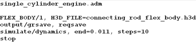
| 4. | Add the following text in line 3 : |
FLEX_BODY/1, H3D_FILE=connecting_rod_flex_body.h3d
The ACF file should look like this:
| 5. | From the toolbar, click the Save Document icon,  , and save the file as single_cylinder_engine.acf to your <working directory>. , and save the file as single_cylinder_engine.acf to your <working directory>. |
| Note | The connecting_rod_flex_body.h3d file that has been used in this tutorial is generated using the FlexPrep utility in MotionView. Refer to the MotionView online help for more information on converting an Adams MNF file into a MotionView H3D flexbody. |
Step 2: Running the ACF file in MotionSolve.
| 1. | Click Start > All Programs > Altair HyperWorks > MotionSolve. |
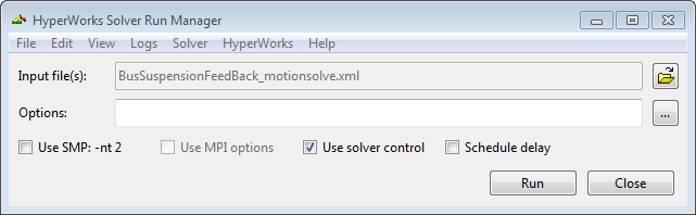
| 2. | For Input file, click Browse and select All files (*.*) from the file type menu. Select the input file single_cylinder_engine.acf from your <Working directory>. |
MotionSolve translates the Adams model (ADM, ACF) to the MotionSolve XML format and solves it. MotionSolve internally invokes OptiStruct, which converts the connecting rod flexbody MNF and MTX files to a flexbody H3D file.
MotionSolve outputs the following files:
| • | Results H3D file - single_cylinder_engine.h3d |
| • | Plot files - single_cylinder_engine.abf and single_cylinder_engine.plt |
| • | Log file - single_cylinder_engine.log |
| Note | MotionSolve is completely integrated into MotionView. You can also use the Run icon,  , from the toolbar in MotionView to perform this action. MotionSolve can also be run from the command prompt. Open a DOS command window, and at the command prompt type: , from the toolbar in MotionView to perform this action. MotionSolve can also be run from the command prompt. Open a DOS command window, and at the command prompt type:
[install_path]\hwsolvers\scripts\motionsolve.bat input_filename.[fem,acf,xml] |
Step 3: View transient analysis results in HyperView by adding external graphics.
Since the ADM file does not carry the external graphic information, the results from MotionSolve will not contain this information either. From Adams, you can export a Parasolid file which can be used for visualizing results in HyperView. In this step, we will attach the piston and crank external graphic for better result visualization.
| 1. | Start a new HyperView session. |
| 2. | Using the Load model file browser,  , select: single_cylinder_engine.h3d, located in your <working directory>. , select: single_cylinder_engine.h3d, located in your <working directory>. |
The Load results file field will be automatically be updated with the single_cylinder_engine.h3d file.
The model is displayed in the window.
| 4. | From the Add Object panel,  , using the Add object from: browser, select the piston.h3d file. If the Add Object icon is not visible on the toolbar, select the View menu > Toolbars > HyperView > Tools. , using the Add object from: browser, select the piston.h3d file. If the Add Object icon is not visible on the toolbar, select the View menu > Toolbars > HyperView > Tools. |
| 5. | For Select object, select All to add all objects to the list. |
| 6. | Using the expansion button,  , select Piston as the component with which you want the selected object to move. , select Piston as the component with which you want the selected object to move. |
| 7. | For Reference system, select the Global coordinate system. |
Notice that the piston graphic is added to the model.
| 9. | Repeat steps 5 through 8 to add the crank object to the model. |
| Note | Remember to select the crank.h3d file in the Add Object from: browser and attach it to Crank using the expansion button. |
| 10. | Click the Contour icon,  , on the toolbar. From the Result type drop-down menu, select the data type that should be used to calculate the contours. , on the toolbar. From the Result type drop-down menu, select the data type that should be used to calculate the contours. |
| 11. | Select a data component from the second drop-down menu located below Result type. |
| Note | If you select Mag (Magnitude), the results system is disabled (since magnitude is the same for any coordinate system). |
The contour is displayed.
| 13. | Click the Start Animation icon,  , on the toolbar to animate the model. , on the toolbar to animate the model. |
| 14. | Click the Stop Animation icon,  , on the toolbar to stop the animation. , on the toolbar to stop the animation. |
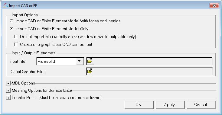
| Note | In the Add Object from: browser, you can directly select a wavefront file (*.obj) from Adams to add graphics. Whereas, if you have a Parasolid file (*.x_t) from Adams, use the Tools menu > Import CAD or FE utility in MotionView to generate an H3D file. You can then use this file to add the graphics. |
Refer to the MotionView help for additional details.


