MV-2020: Use of Flexbody in MBD Models

In this tutorial you will:

•	use the flexible bodies created in tutorial MV-2010 in an MBD model and solve the model using MotionSolve.

Exercise: Simulating a Front SLA suspension with Flexible LCA

Step 1: Replacing rigid bodies with flexible bodies and solving them in MotionSolve.

In this exercise, you will integrate the flexbodies into your MBD model.

1.	From the MotionView menu bar, select Model > Assembly Wizard… to bring up the wizard.

2.	Use the criteria from the table below to assemble a front end half vehicle model.

Panel	Selection
Model Type	Front-end of the vehicle
Driveline Configuration	Defaults <No driveline>
Primary Systems	Front Suspension = Frnt. SLA susp (1 pc LCA) and defaults for the rest
Steering Subsystems	Steering Column = Steering column 1 (not for abaqus) and Steering boost = None
Springs, Dampers, and Stabars	Defaults
Jounce/Rebound Bumpers	Defaults
Label and Varname	Defaults
Attachment Wizard	Compliant = Yes; Defaults for the rest

Assembly Wizard settings

You should make sure to select Frnt. SLA susp (1 pc LCA) since the flexible bodies you have created are for this suspension geometry.

3.	From the MotionView menu bar, select Analysis >Task Wizard… to display the wizard.

4.	Load a Static Ride Analysis task from the Task Wizard - Front end tasks. Click Next and click Finish.

5.	The Vehicle Parameters form is displayed. Click Finish.

6.	From the Project Browser, select Lwr control arm from the Bodies folder (located underneath the FrntSLA Susp (1 pc.LCA) system).

The Bodies panel is displayed.

7.	Under the Properties tab for the Lwr control arm-left, deselect the symmetry check-box, Symmetric properties.

8.	The Remove Symmetry confirmation dialog is displayed. Click Retain to retain the current values of properties of Lwr control arm-right.

9.	Select the Flex Body (CMS) check box and click Yes to confirm both sides as deformable.

mv-2020-a

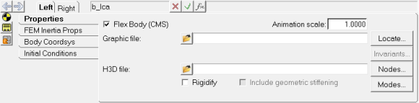
Notice that the graphics of the rigid body lower control arm vanishes.

10.	Using the Graphic file browser, , select the file sla_flex_left.h3d (created in earlier tutorial MV-2010) from your working directory.

11.	You will see that the H3D file field is populated automatically with the same path and the file name as the graphic file you specified in point 10.

mv-2020-b

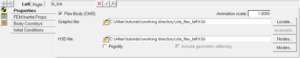
Properties panel

The flexible body drops into the right position.

Note	You need to specify the flexbody H3D file as the H3D file. Specify the same or any other file as the Graphic file.

External Graphics for Flexbodies

Use of large flexbodies is becoming very common. For faster pre-processing, you can use any graphic file for the display and use the flexbody H3D file to provide the data to the solver. You can use the input FEM deck or the CAD file used for the flexbody generation to generate a graphic H3D file using the CAD to H3D Conversion and specify that file as the Graphic file. This will make pre-processing a much more efficient process.

Locate Feature

The Locate button on this panel is an optional step to relocate a flexible body if it is not imported in the desired position. This may happen if the coordinate system used while creating the flexible body in the original FEM model does not match the MBD model coordinate system. However, if your flexible body is already in the desired position, you can skip this step.

12.	Click Nodes….

The Nodes panel is displayed.

mv-2020-c

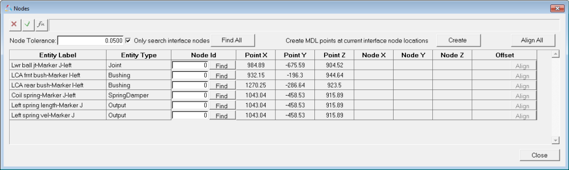
The Nodes panel is used to resolve the flexbody’s attachments with the vehicle model, since the vehicle model is attached to the flexible body at these interface nodes.

This panel lists all markers of the connections (joints/forces)on the body which is now flexible. These markers can interact with the flexible body only through a node. This panel is used to map each of the markers to a node. The panel also displays the point coordinates of the marker origin which are nothing but coordinates of a point entity that the connections are referring to.

13.

Click the Find All button on the Nodes dialog to find nodes on the flexible body that are located closest to the interface points on the vehicle model. Node ID column is populated with the interface node numbers for each row of connections. Also, the node coordinate table is also populated along with the Offset with respect to the point coordinates.

14.	Observe a small offset for the Lwr ball jt-Marker J-left. It suggests a difference in the coordinate values between the point at which the joint Lwr ball jt is defined and its corresponding location of the interface node 10004. Click Align to move the point to the nodal coordinate position.

Note

Many times there is a little offset between the flexible body interface node and its corresponding point in the model. When you click the Align button, MotionView moves the connection point in the model to the node location on the flexible body. This could affect other entities that reference this point. Hence, this option should be used with caution. Generally, it is common to have minor offsets (values between 0.001mm to 0.1mm). If the offset is more than the tolerance value, MotionView inserts a dummy body between the flexible body and the nearest connection point. If the offset value is too high, it could indicate an mismatch of the FE model information with respect to the MBD model. In such an event, it is recommended to review the models and reconcile the differences.

15.	Close the Nodes dialog.

16.	Click the Modes button. The Modes panel is displayed. This option lets you select the modes that will be active during the simulation. By default, the rigid body modes are deactivated. You can also change the damping used for modes.

mv-2020-e

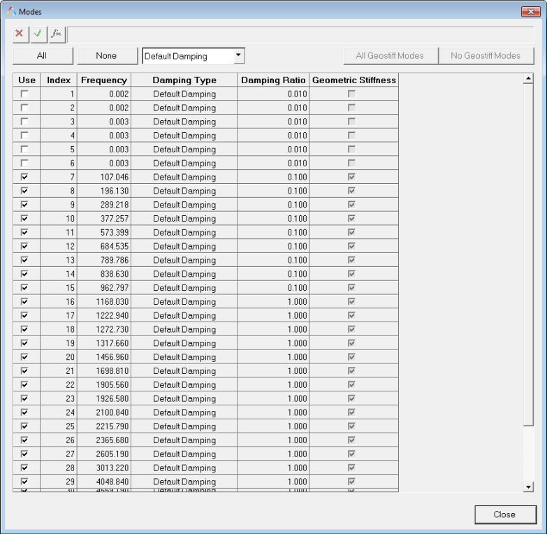
Note	By default, for frequencies under 100Hz, 1% damping is used. For frequencies greater than 100Hz and less than 1000Hz, 10% damping is used. Modes greater than 1000 Hz use critical damping. You can also give any initial conditions to the modes.

Please note that when selecting the modes, the simulation results may vary as you change the modes to be included in the simulation.

17.	Click Close.

18.	Repeat steps 7 through 17 to integrate the right side flexible body sla_flex_right.h3d (created in tutorial MV-2010) in your model.

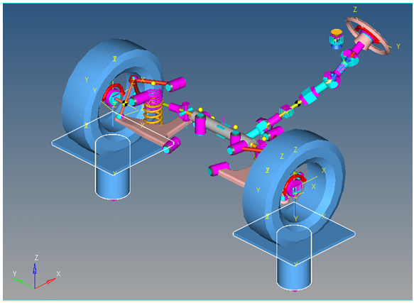
Your model should look like the image below:

mv-tut_bmct_mv-2020-f

Now you will review the properties of the FEM model file.

19.	Click the FEM Inertia Props tab.

The following information is displayed:

mv-2020-g

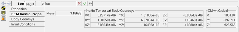
Bodies panel/FEM Inertia Props tab

20.	From the Tools menu, select Check Model to check your complete MBD model for errors.

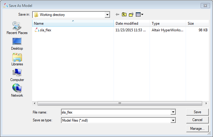
21.	From the Standard toolbar, click the Save Model icon, , to save your model as an MDL file named sla_flex.mdl.

The Save As Model dialog is displayed.

mv-2020_savemodel

22.	Click the Run icon, , on the toolbar and run the model with simulation type Quasi-Static, specifying the filename as sla_flex_ride.xml.

23.	Once the run is complete, load the MotionSolve result file sla_flex_ride.h3d (located in your working directory) in a HyperView window and view the animation of the run.