pressures panel

Use the Pressures panel to create pressure loads on elements by applying a load, representing pressures, to a 1D or 2D element, or to the face of a solid element.

For most solvers, the pressure load is considered as force/area, therefore the magnitude of the pressure is multiplied by the calculated area of the elements to which it is applied and resolved as concentrated force loads at the associated nodes. Refer to solver documentation for the specific details on how these load types are handled.

Pressures are load config 4 and are displayed as a vector with the letter P at the tail end. By default, pressures are displayed relative to the model size. You can change this size by entering a different value in the relative size field. You can also use the uniform size option to display all loads with the same size. Finally, you can remove the on-screen text labels of all pressures by deactivating the label loads checkbox.

Panel Usage

The Pressures panel consists of two subpanels. Switching from one subpanel to the other will not clear any data entered in either panel. Once criteria are set in a subpanel, pressures are created, rejected, or reviewed by means of a column of buttons along the left-hand side of the subpanel.

pressures_panel

Subpanels and Inputs

The Pressures panel contains the following subpanels and command buttons:

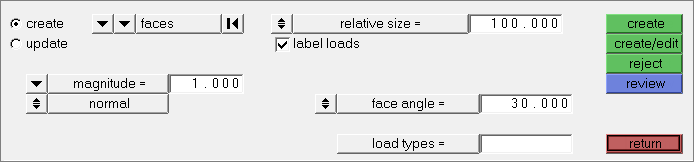
Use the Create subpanel to create new pressures. You can specify the pressure's footprint by picking the elements it affects, as well as its direction, magnitude, and the size in which its visual indicators are drawn. You can also apply the pressure to the faces of solid elements, or to the edges of plate elements.

For plate elements, the pressure is applied along the positive element normal. The Normals panel should be used first to obtain the correct orientation. The nodes on face option is not necessary if applying the pressure to the face of a plate element. If applying the pressure to the edge of plate elements, the nodes on edge option is required to define which of the three or four edges of the plate element you wish to apply the pressure to.

For solid elements, the nodes on face option is required to define which of the faces you wish to apply the pressure to.

Panel Inputs

Input

Action

elems selector

Select elements (1D, 2D, 3D) to apply pressure to.

Use the switch to change the selection mode.

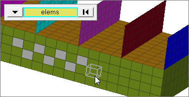
elems

Select individual elements, or select all of the elements contained by a component or on a surface.

faces_edges_entities

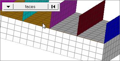
faces

Select all of the elements on 2D and 3D faces.

If there are discontinuities on a 2D face, then only the elements inbetween the discontinuities will be selected.

faces_edges_faces

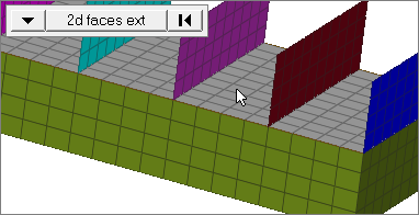
2D faces ext

Select all of the elements on a 2D face that contain discontinuities.

faces_edges_2d_faces_ext

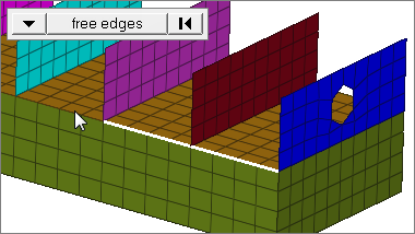
free edges

Select all of the free edges of elements.

If there are discontinuities on an edge, then only the free edges of elements inbetween the discontinuities will be selected.

Only valid for SHELL elements.

faces_edges_free_edges

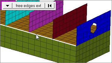
free edges ext

Select all of the free edges of elements that contain discontinuities.

Only valid for SHELL elements.

free_edge_ext

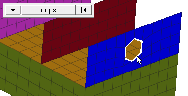
loops

Select all of the continuous free edges of elements that make a closed loop simultaneously, such as the perimeter of a hole.

Only valid for SHELL elements.

faces_edges_loops

Note:

If you leave the pressure panel, your current selection will disappear, but it will be restored once you return to the panel.

Changing the selection mode will clear your current selection. Use the Entity Editor to select elements using multiple selection modes.

magnitude =

This switch actually presents a very different set of options depending on what you pick:

•	magnitude (constant vector): Specify a numerical magnitude for the pressure.

•	constant components: Specify the X, Y, and Z components; the resulting pressure vector will be derived from these components.

•

curve, vector: This option for pressures that are time-dependent lets you specify the time history of the pressure using a vector entity.
When using this option, you may choose to apply the pressure normal to the elements, or use the plane and vector selector to specify a direction.
The curve selector is used to select the curve representing the load time history. This curve must already exist in the model.
The optional scale factor field allows you to scale the X vector of the curve.
Curves can be viewed and modified from within the XY Plots module.

•

curve, components: Type in the X, Y, and Z components to define the direction and magnitude--for example, (2,2,2) will be twice the magnitude of (1,1,1). Next, click the curve field twice to select from a list. Finally, specify a factor for the curve’s xscale.
Curves can be viewed and modified from within the XY Plots module.

•	equation: type the loading equation into the entry field that displays.

Equations allow you to create force, moment, pressure, temperature or flux loads on your model where the magnitude of the load is a function of the coordinates of the entity to which it is applied. An example of such a load might be an applied temperature whose intensity dissipates as a function of distance from the application point, or a pressure on a container walls due to the level of a fluid inside.

Functions must be of the form magnitude= f(x,y,z). The only variables allowed are x, y and z, (lower case) which are substituted with the coordinate values of the entity to which the load is applied. In the case of grid point loads (force, moment or temperature) the grid point coordinates are used. For elemental loads (pressure or flux) the element centroid coordinates are used. In the event that a cylindrical or spherical coordinate system is used, x, y and z are still used to reference the corresponding direction. Standard mathematical operators and functions can be used; however, any functions requiring external data will not be valid. See Functions and Operators for a complete list.

Note:

If your equation contains a syntax error, no warning message will be displayed, but any loads created will have a zero magnitude.

Examples:

A flat plate, 20 x 20 units, lying in the X-Y plane with the origin at the center. A linear function for an applied force
magnitude = 20 – (5*x+2*y):

load_equations_ex1

The same plate with a polynomial function

magnitude = x^2-2y^2+x*y+x+y:

load_equations_ex2

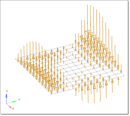
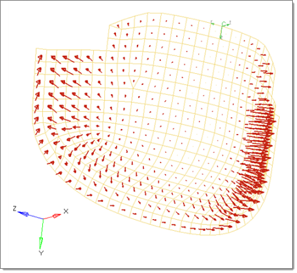
A curved surface with a polynomial function for an applied pressure magnitude = -((x^2+2*y^2+z)/1000). The pressure function is defined in terms of the cylindrical coordinate system displayed at the top edge of the elements.

load_equations_ex3

Optionally, you can also use the plane and vector selector to specify a direction, and select the coordinate system to which the vector corresponds.

Then choose to apply the pressure normal to the elements, or use the plane and vector selector to specify a direction.
Optionally, specify a coordinate system that the pressure is aligned to; if not specified, the global system us used by default.

•	Linear interpolation: Use this option to interpolate pressures from a saved file or existing loads.

Note:

Linear interpolation only works with shell elements.

Each row of the input file contains the pressure's x,y,and z coordinates followed by its magnitude. Loads that are formatted in CSV (Comma Separated Values) files or SSV (Space-Separated Values) text files can be interpolated.

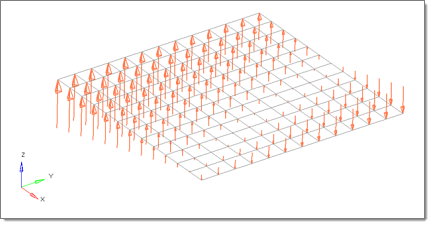
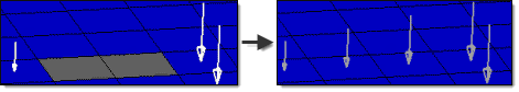
You can then select the desired elements to which you wish to add loads, and pick 3 or more existing loads that enclose those elements. When you interpolate, a linear function is used to create additional loads on the selected elements, with magnitudes based on the magnitudes of the loads that you had selected:

pressures_linearinterpolate

The search radius is a search distance to find the loads which are within that distance from a centroid or node on which a load is being interpolated. The nearest 3 loads located within that distance are used to create the load at the centroid or node by linear interpolation. Linear interpolation uses a triangulation method, so if it finds fewer than 3 loads within that distance no interpolation takes place. While reading the initial loads from a file, if linear interpolation is not possible because the search radius is too small, the original loads are simply applied to the nearest centroid or node.

•

To interpolate and extrapolate pressures from existing loads, select field loads. You can then select the desired elements to which you wish to add loads, and any existing loads on which you wish to base additional forces. Field Loads will not overwrite any existing loads, so you can create an area of loads via linear interpolation and then use field loads to expand the load area without changing the loads already inside of the area.

When you create, HyperMesh uses a Green’s function with the given boundary loads in order to create the loads on all of the selected elements. For smoothness, the gradient at the boundary points is enforced to be zero. This ensures that the extrapolated loads remain lower than the input loads. For this reason it is recommended to use representative boundary values as input to be able to capture the peaks reasonably.

Note:

This version differs from linear interpolation both in the way that the load magnitudes are determined, and also in the fact that it can be applied to elements outside the boundaries of the chosen existing loads.

•	fill gap: When "fill gap" is checked, a load is created at every selected element centroid or node irrespective of the size of the search radius.

normal / N1,N2,N3

The created pressure will be in the positive normal direction as determined by the normals of the chosen elements. Alternatively, pick three nodes to define a plane; the pressure is applied in the positive normal direction of that plane as determined via the right-hand rule.

relative size / uniform size

This setting does not affect the pressure load, only the length of its graphical indicators. Use the toggle to choose between these options, then type in a numeric value.

•	relative size = display pressures in a size relative to the model size (default 100).

•	uniform size = display all pressures with the same size.

label loads

When this checkbox is active, text labels for each of the loads display in the graphics area.

nodes on face / nodes on edge

To apply pressures to the face of a solid element, set the toggle to nodes on face. The face or edge nodes define the starting face or edge. For a four-noded face, pick the diagonally opposing nodes. For a three-noded face, pick all of the nodes.

•	You can select a surface that represents the faces you want the loads to be applied to. This places loads on the faces of all elements associated with the selected surface.

•	Alternatively, select the nodes representing the face of the solid element the load is to be applied to.

If the pressure is being applied to the edge of an element for an axisymmetric problem, set the toggle to nodes on edge:

•	You can select the nodes that represent the edge of the element you want the load on, or the lines that represent the edges of all the elements that you want to place loads on.

Only available when the selector is set to entities.

face angle / individual selection

Face angle

Value used to determine which of the selected elements are to have pressures applied. For pressures applied to faces, once the starting face has been identified, the normals of the adjacent remaining faces are tested. If the angle between the normals is less than the face angle, a pressure is applied to the adjacent element. This process continues until all of the free faces have been tested. For a pressure applied to edges, the process is similar except that the angle between edges is used instead of the angle between faces.

Only available when the entity selector is set to elems and the selection mode is set to faces, 2d faces ext, free edges, or free edges ext.

Individual Selection

Select individual elements on a face or select individual free edges of elements.

Only available when the entity selector is set to elems and the selection mode is set to faces or free edges.

edge angle

Splits edges that belong to a given face.

When the edge angle is 180 degrees, edges are the continuous boundaries of faces. For smaller values, these same boundary edges are split wherever the angle between segments exceeds the specified value. A segment is the edge of a single element.

Only available when the entity selector is set to elems and the selection mode is set to free edges or free edges ext.

load types =

Click this field to open a pop-up menu of available load types to apply to the pressure. Available types depend on the current solver profile.

Use the Update subpanel to alter existing pressure loads. You can pick the desired loads and edit their magnitude, direction, visual indicator draw size, and load type.