HM-4350: Pre-Processing for Crashing Tubes Analysis using Abaqus

For this tutorial it is recommended that you complete the introductory tutorial, HM-1000: Getting Started with HyperMesh as well as the tutorial HM-4310: Defining Abaqus Contacts for 2-D Models in HyperMesh. Working knowledge of the creation and editing of collectors and card images are a pre-requisite.

In this tutorial you will learn how to setup an Abaqus input file in HyperMesh, which will be used to obtain the dynamic response of multiple tubes with one tube fully constrained, and gravity applied on the other tubes. The modeling steps that are covered are:

•	Create *ORIENTATION system

•	Create contact between shell elements

•	Create a step with AMPLITUDE associated to DLOAD

The units used in this tutorial are Milliseconds, Millimeters, Kilograms, and Kilonewtons (ms, mm, kg, kN), and the tutorial is based on Abaqus 6.9-EF1.

For more information regarding the panels used in this tutorial, please refer to the Panels section of the on-line help, or click the h key while in the panel to bring up its context sensitive help. For detailed information on the HyperMesh Abaqus interface, refer to the External Interfacing section of the on-line help.

This tutorial requires about 30 minutes to completed.

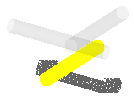
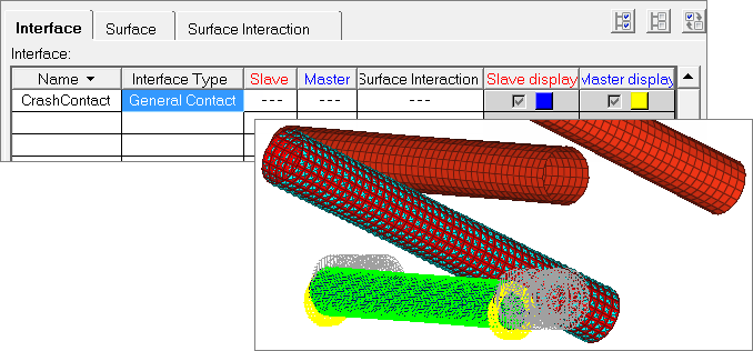
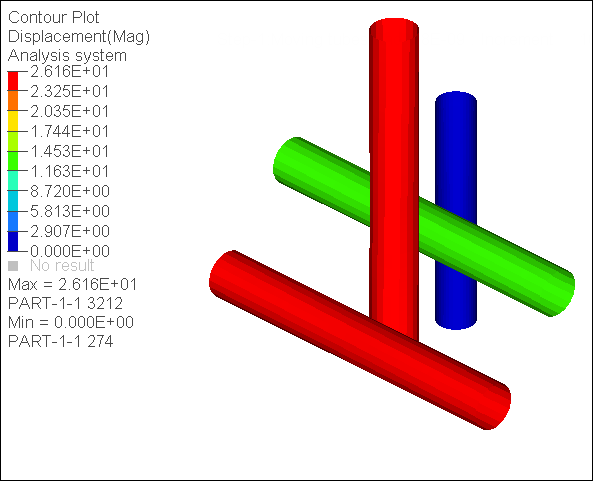
The model used is composed of four tubes (see image below).

HM-4350-01

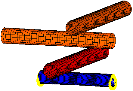
Crashing tubes

Model Files

This exercise uses the crash_tubes.hm file, which can be found in <hm.zip>/interfaces/abaqus/. Copy the file(s) from this directory to your working directory.

Exercise

Step 1: Load the Abaqus Explicit user profile and retrieve the model

1.	Start HyperMesh Desktop.

2.	In the User Profile dialog, set the user profile to Abaqus, Explicit.

3.	Open a model file by clicking File > Open > Model from the menu bar, or clicking on the Standard toolbar.

4.	In the Open Model dialog, open the crash_tubes.hm file. The model contains the following Abaqus model and history data:

•	Four tubes with shell (S4R) elements. The corresponding ELSETs are named FixTube, MovTube, MovTube2 and MovTube3.

•	A *SHELL SECTION property for each tube. Each property is associated with one of two materials.

•	*BOUNDARY constraints on the ELSET named FixTube.

•	A HyperMesh system.

Defining the Abaqus *ORIENTATION in HyperMesh

*ORIENTATION specifies a local system defining local material directions for elements.

In Abaqus, shell and membrane elements have default local directions. They are not the global system directions. The default local 1-direction is the projection of the global x axis direction onto the shell surface. If the global x axis is normal to the shell surface, the local 1-direction is the projection of the global z axis onto the shell surface. The local 2-direction is perpendicular to the local 1-direction in the surface of the shell. Refer to the figure below.

HM-4350-02

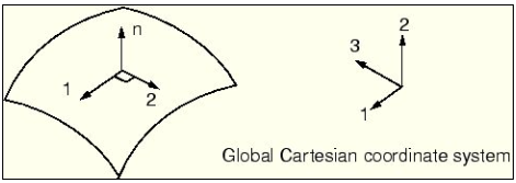
Default local shell directions

The general steps outlined below can help you understand the process followed in this tutorial.

1.	Create a System Collector with no card image and give it a name as per your preference.

Note:

Any number of systems can be collected in a system collector.

2.	Create a system by clicking Geometry > Create > System from the menu bar.

3.	Create the *ORIENTATION using the Card panel.

4.	In the Card panel, select the HyperMesh system (systs) and click edit.

5.	Activate the ORIENTATION option to create the *ORIENTATION keyword.

If the *ORIENTATION system is for solid elements, do not activate the locdir_alpha option. If this *ORIENTATION system is for shell and membrane elements, activate the locdir_alpha option. By default, the local axis closest to being normal to the elements’ 1 and 2 material directions is the local 1-axis. Also by default, the additional rotation about the local normal axis is 0. You can change these values by editing the [locdir] and [alpha] fields in the pop-up card image.

7.	Associate the *ORIENTATION to the desired sectional properties.

Local directions for this model

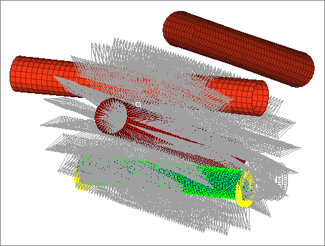
The default set of local material directions can sometimes cause problems; a case in point is the model’s fixed tube pictured below. For most of the elements in the tube, the local 1-direction is circumferential. However, there is a line of elements normal to the global x axis. For these elements the local 1-direction is the projection of the global z axis onto the shell, making the local 1-direction axial instead of circumferential. A contour plot of the direct stress in the local 1-direction will look strange, since for most elements, it is the circumferential stress, whereas for some elements it is the axial stress. In this case, use the *ORIENTATION option for the fixed tube to define more appropriate local directions.

HM-4350-03

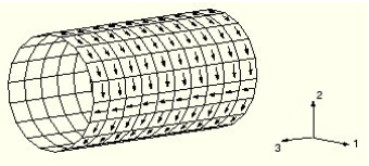
Default local 1-direction in the fixed tube

Step 2: Create the *ORIENTATION for the fixed tube

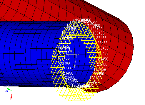
In this step, you will use the approach described in the previous section to create an *ORIENTATION for the fixed tube. Use the pre-defined cylindrical coordinate system for this tube and define the card using the Card panel.

1.	Use your mouse to position the model to the view shown below. This system is located at one end of the fixed tube and is organized in the system collector.

HM-4350-04

2.	From the menu bar, click Geometry > Card Edit > Systems to edit the system's card and define the *ORIENTATION option.

3.	Using the systs selector, select the local system.

4.	Click edit.

5.	In the Card Image, select the ORIENTATION checkbox.

6.	In the *ORIENTATION, NAME field, enter Orient_Coord.

hm-4350-06

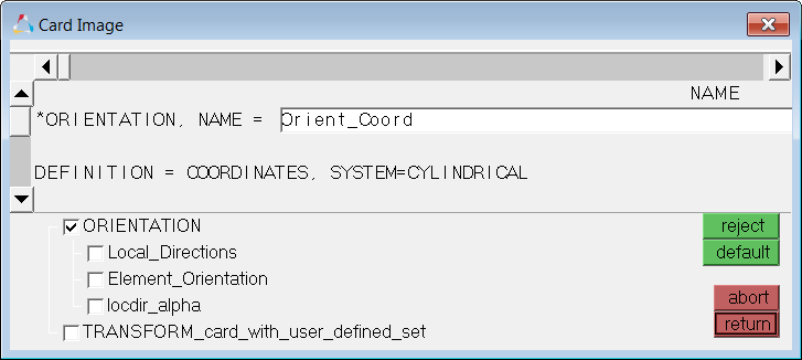
7.	Select the locdir_alpha checkbox. The locdir and alpha fields display under *ORIENTATION in the card image.

Tip:	Use the vertical scroll bar to display the locdir and alpha parameters if they are not visible.

hm-4350-07

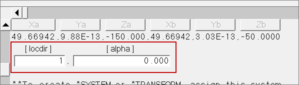
8.	Leave the locdir field set to 1 to specify the radial axis as the axis closest to being normal to the shells’ 1 and 2 material directions.

9.	Leave the alpha field set to 0 for the additional rotation of the local normal axis.

10.	Click return to close the card image.

11.	In the card editor, set the entity selector to props.

12.	Click props.

13.	Select the property, FixTube.

14.	Click select. *ORIENTATION is now associated with the fixed tube's sectional property.

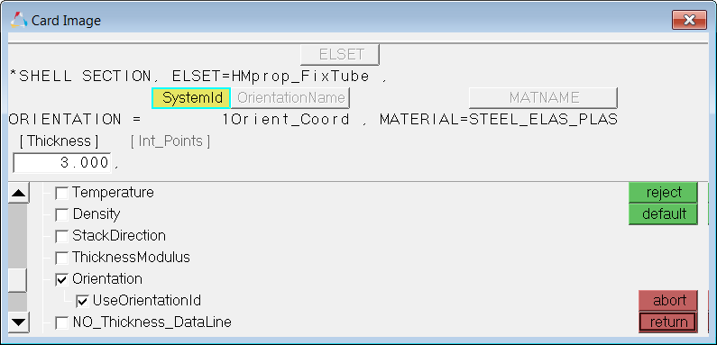
15.	Click edit. The Card Image opens, and displays *SHELL SECTION, ELSET = FixTube.

16.	Select the Orientation checkbox.

17.	Select the UseOrientationId checkbox.

18.	Click the SystemId selector and graphically select the system. This method also assigns the system name to the card image.

hm-4350-08

19.	Click return to close the card image.

20.	Click return to exit the panel.

*ORIENTATION has now been defined for ELSET FixTube.

Step 3: Define contact between the tubes as Abaqus general contact

General contact is usually easier to set up than common contact between two surfaces. Follow the steps below to set up a general contact.

The following is the simplest definition of general contact:

*CONTACT

*CONTACT INCLUSIONS, ALL EXTERIOR

You can assign other contact properties within a general contact using the following option.

*CONTACT PROPERTY ASSIGNMENT

surf_1, surf_2, prop_1

In this section, you will use the Contact Manager to define a contact pair property between the FixTube and the MoveTube (the closest tube to the fixed tube). Then you will define a general contact for the entire model and assign the contact pair property to it.

The general contact algorithm is used to define contacts between the tubes. A contact pair property is assigned to the general contact to define a different type of contact algorithm between the FixTube and the MoveTube. This contact pair property is not required. However, it is created here for the purpose of demonstrating how it is specified in a general contact using HyperMesh.

In a model like this, where both components have similar geometry (mesh) and material properties, either the fixed or moving tube can be chosen for the slave or master surface. Here use the ELSET FixTube for the slave surface of the contact pair property.

Complete the steps below to create a slave *SURFACE on FixTube by selecting elements in the Contact Manager:

1.	From the menu bar, click Tools > Contact Manager. The Contact Manager opens.

hm-4350-09

2.	Click the Surface tab.

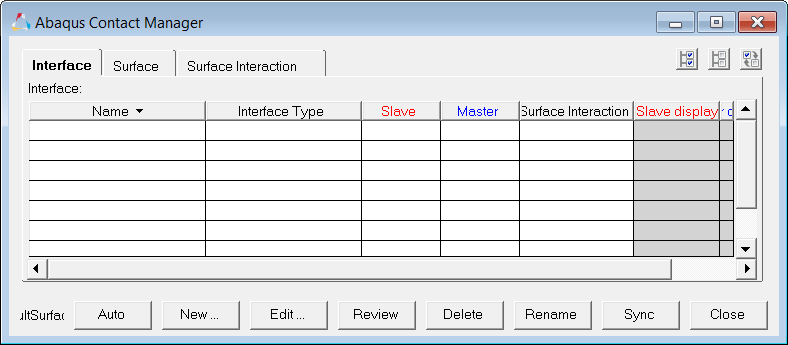
3.	Click New to define a surface.

4.	In the Create New Surface dialog, Name field, enter S1_Fixed.

5.	Leave the surface Type set to Element based.

6.	Optional. Choose a Color for visualizing the surface.

hm-4350-10

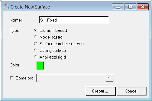
7.	Click Create. The Element Based Surface dialog opens.

8.	In the Define tab, set Define surface for to 3D shell, membrane, rigid.

9.	Click Elements to select the elements on which the surface will be defined.

10.	In the panel area, click elems >> by collector.

11.	Select the component, FixTube.

12.	Click select.

13.	Click proceed. The normals for the selected elements display. The normals should be pointing out of the fixed tube, which indicates the desired direction.

14.	Optional. SPOS will be written to the input file for the elements in this contact surface. Specify SNEG in the input file by selecting the Reverse checkbox in the Contact Manager before going to the next step. This does not change the element normals.

15.	Click Add to add the elements to the surface.

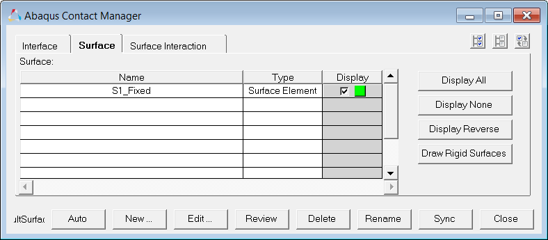
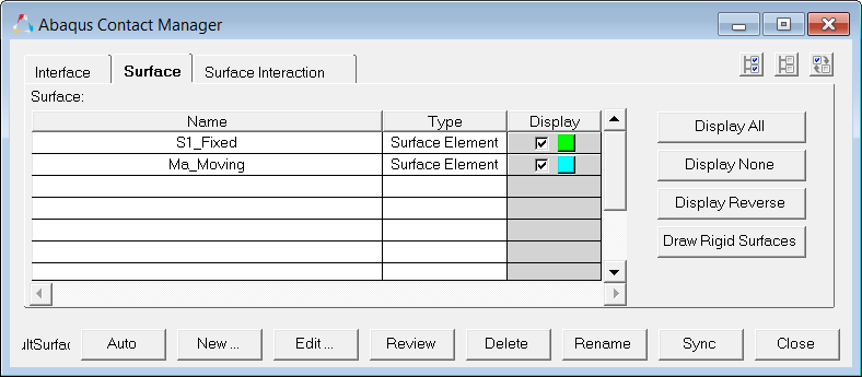
16.	Click Close to return to the Contact Manager. Notice the surface Sl_Fixed is now listed in the Surface tab.

hm-4350-11

Step 4: Create master *SURFACE on MoveTube by selecting a set of elements in the Contact Manager

1.	In the Surface tab, click New to begin defining a second surface.

2.	In the Create New Surface dialog, Name field, enter Ma_Moving.

3.	Leave the surface Type set to Element based.

4.	Optional. Select a Color for visualizing the surface.

5.	Click Create. The Element Based Surface dialog opens.

6.	Set Define surface for to Element set.

7.	Set Element set to Ma_TubeContSet.

8.	Click Review Set. The elements in the selected set highlight.

hm-4350-12

9.	Return the elements to their original color by right-clicking on Review Set.

10.	Click Show Faces to view the direction of the element normals. The normals should be pointing into the moving tube, which indicates the faces on the inside of the moving tube elements are SPOS.

hm-4350-13

11.	In the Element Based Surface dialog, click on the right arrow key to move the Ma-TubeContSet element set into the table.

hm-4350-14

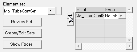
12.	In the Face column, click the pull down-menu and select SNEG.

This specifies the faces on the outside of the moving tube elements. SNEG is written to the input file for the set of elements forming this master contact surface.

13.	Select the Display checkbox, then click Update.

14.	In the Confirm dialog, click Yes.

15.	Click Close to return to the Contact Manager. Notice the surface Ma_Moving is now listed in the Surface tab.

hm-4350-15

Step 5: Create *SURFACE INTERACTION in the Contact Manager

1.	In the Contact Manager, click the Surface Interaction tab.

2.	Click New to create a new surface interaction.

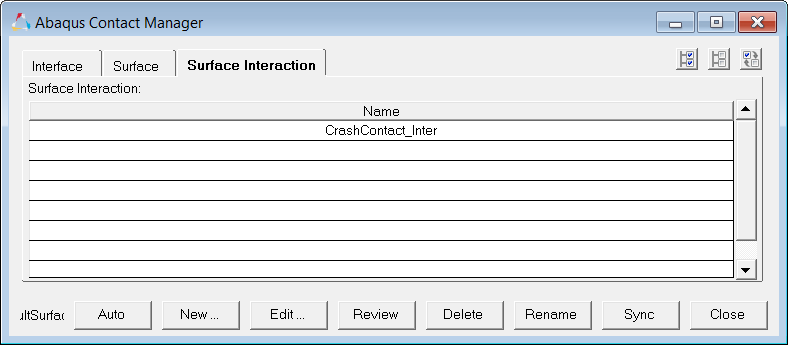
3.	In the Create New Surface Interaction dialog, Name field, enter CrashContact_Inter.

4.	Click Create. The Surface Interaction dialog opens.

5.	In the Define tab, select the Friction checkbox.

6.	Click the Friction tab.

7.	In the table at the bottom of the dialog, enter 0.2 in the Friction Coeff column.

8.	Click OK to return to the Contact Manager. Notice the surface interaction CrashContact_Inter is now listed in the Surface Interaction tab.

hm-4350-16

Step 6: Define a general contact *CONTACT in the Contact Manager

1.	In the Contact Manager, click the Interface tab.

2.	Click New to define a new interface.

3.	In the Create New Surface dialog, Name field, enter CrashContact.

4.	Set Type to General Contact.

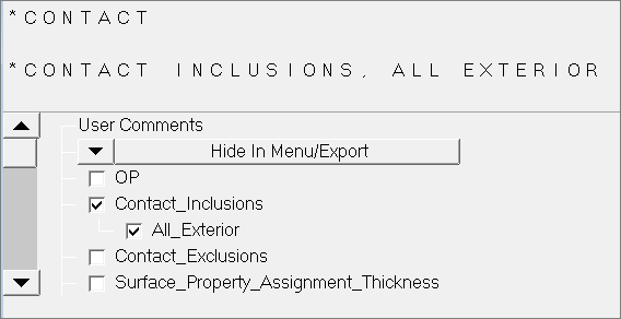
5.	Click Create. The Card Image opens with *CONTACT shown.

6.	Select the Contact_Inclusions checkbox to create *CONTACT INCLUSIONS.

7.	Select the All_Exterior checkbox.

hm-4350-17

8.	Select the Contact_Property_Assignment checkbox to create *CONTACT PROPERTY ASSIGNMENT.

Tip:	Use the vertical scroll bar to display the Contact_Property_Assignment parameter if it is not visible.

9.	Double-click the Surface1(1) selector.

hm-4350-18

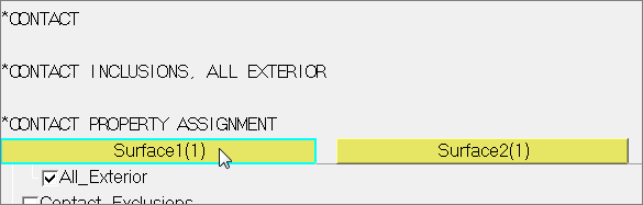
10.	Select the surface, S1_Fixed.

11.	Double-click the Surface 2(1) selector.

12.	Select the surface, Ma_Moving.

13.	Double-click Surface_Interaction(1).

Tip:	Use the horizontal scroll bar to display the Surface_Interaction(1) selector if it is not visible.

hm-4350-19

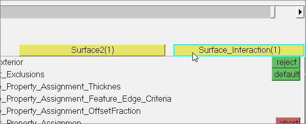
14.	Select the interface, CrashContact_Inter.

15.	Click return to return to the Contact Manager.

16.	Click Close to close the Contact Manager.

Defining the general contact between the tubes is complete.

hm-4350-20

Step 7: Create *STEP

For this analysis, only one *STEP is needed. You will create a *DYNAMIC, EXPLICIT step and specify field output requests. Lastly, you will add the general *CONTACT and *SURFACE INTERACTION (groups) to the step. Adding the latter is required for Abaqus/Explicit, but not Abaqus/Standard. It is history data for Explicit.

1.	From the menu bar, click Tools > Load Step Browser. The Step Manager opens.

2.	In the Step tab, click New to begin defining a step.

3.	In the Create New Step dialog, Name field, enter Crash.

4.	Click Create.

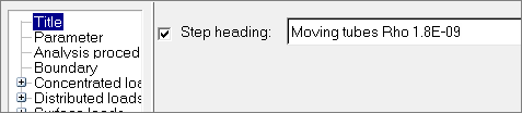
5.	In the first pane, click Title.

hm-4350-21

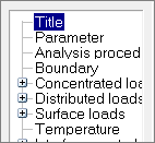
6.	Select the Step heading checkbox, then enter Moving tubes Rho 1.8E-09.

hm-4350-22

7.	Click Update.

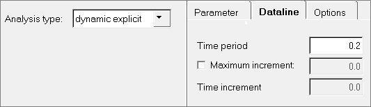
8.	In the first pane, click Analysis procedure.

9.	Set Analysis type to dynamic explicit. Additional tabs appear.

10.	Click the Dataline tab.

11.	In the Time period field, enter 0.2.

hm-4350-23

12.	Click Update.

13.	Close the Step Manager.

Understanding boundary conditions for this model

In Abaqus/Standard, common boundary conditions are *BOUNDARY constraints to prevent rigid body motion and *CLOAD and *DLOAD (forces and pressures). In Abaqus/Explicit, common boundary conditions are constraints and time varying boundary conditions, like time varying displacement, velocity or acceleration, causing dynamic structural response.

For this analysis, the nodes at the ends of the fixed tube are fully constrained with *BOUNDARY constraints. These *BOUNDARY constraints are model data. In HyperMesh, they are organized into a load collector named "Constraint" with the card image INITIAL_CONDITION.

*DLOAD, TYPE = GRAVITY, AMPLITUDE = curve will be created for all nodes of the moving tubes. This is a constant acceleration applied in the global x direction. *AMPLITUDE is not required for gravity since it has a constant magnitude. However, *AMPLITUDE is assigned to the *DLOAD in this section for the purpose of showing you how to do this in HyperMesh. *AMPLITUDE allows arbitrary time variations of the applied condition throughout a step.

Step 8: Create *AMPLITUDE in HyperMesh

*AMPLITUDE is an xy curve in HyperMesh. There are two methods for creating *AMPLITUDE in HyperMesh.

Method 1:

Create *AMPLITUDE using the Curve Editor, which can be accessed by clicking XY Plots > Curve Editor from the menu bar. This is a quick and easy way to create new AMPLITUDE cards.

Method 2:

Create plots and curves by clicking XY-Plots > Create > Plots or Curves from the menu bar. This method provides additional functionalities, such as reading data from a file or generating curves by simple math. Please refer to XY Plotting in the online documentation for more information.

HyperMesh supports *AMPLITUDE with DEFINITION = TABULAR, EQUALLY SPACED and SMOOTH STEP. Use the Step Manager to associate a *AMPLITUDE to a load in HyperMesh.

Complete the steps below to create *AMPLITUDE in the Curve Editor.

1.	From the menu bar, click XYPlots > Curve Editor. The Curve Editor opens.

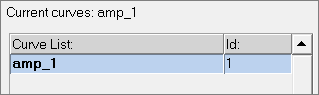
2.	Click New to create a new curve.

3.	In the panel area, enter amp_1 in the Name field.

4.	Click proceed.

5.	From the Curve List, select amp_1 to activate the new curve.

hm-4350-24

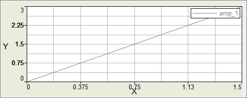
6.	In the X, Y table, enter the following values.

Tip:	You can also copy and paste values column by column from a spreadsheet.

X	Y
0.0	0.0
0.5	1.0
1.0	2.0
1.5	3.0

7.	Click Update. The new amplitude curve displays.

hm-4350-25

8.	Click Close.

Step 9: Define *DLOAD, TYPE = GRAVITY

In this step you will define *DLOAD, TYPE=GRAVITY on all of the nodes of the moving tubes using the Step Manager for the step named Crash.

1.	From the menu bar, click Tools > Load Step Browser. The Step Manager opens.

2.	In the Step tab, click the step Crash.

3.	Click Edit. The Load Step dialog opens.

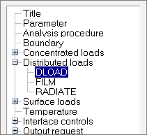
4.	In the first pane, expand Distributed loads, and click DLOAD.

hm-4350-26

5.	Click New.

6.	In the Create Load Collector dialog, Name field, enter GRAVITY.

7.	Optional. Select a display Color for the GRAVITY load collector.

8.	Click Create.

9.	In the Load collector table, click GRAVITY to make the collector active.

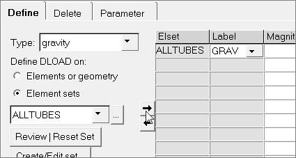
10.	In the Define tab, set Type to gravity.

11.	Set Define DLOAD on to Element sets.

12.	Set Element sets to ALLTUBES.

Tip:	Click to view the enhanced browser, which provides filtering and sorting options for easier selections.

13.	Click the right-arrow button to add the ALLTUBES set to the table.

hm-4350-27

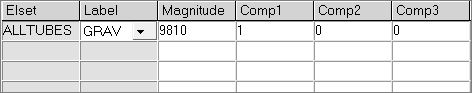
14.	In the Magnitude column, enter 9810.

15.	Enter 1, 0, 0 in the table for Comp1, Comp2, Comp3 respectively. These values define a unit vector in the global x direction.

hm-4350-28

16.	Click Update.

17.	Click the Parameter tab.

18.	Select the Amplitude curve checkbox, then select amp_1.

19.	Click Review/Edit \| Reset.

20.	Click Close to close the Curve Editor.

21.	Click Update to update the step and write the changes to the database.

Step 10: Define output requests for the ODB file

In this step, you will use the Step Manager to define an output request for the step Crash.

1.	In the first pane of the Load Step dialog, expand Output request, and click ODB file.

2.	Click New.

3.	In the Create Output block dialog, Name field, enter field_output.

4.	Click Create.

5.	In the Output block table, click field_output to make it active.

6.	In the Output tab, select the Output checkbox and set it to field.

7.	Select the Node output and Element output checkboxes.

8.	Select the Time marks checkbox, and set it to yes.

9.	Select the Number interval checkbox, and specify 20 intervals.

10.	Click Update.

11.	Click the Node Output tab.

12.	From the list of output options, expand Displacement, and select U to request nodal displacement output.

13.	Click Update.

14.	Click the Element Output tab.

15.	From the list of output options, expand Section_points > O, and select 0, 1, 2, 3, 4, and 5 to request results on element layers 1 through 5.

16.	Expand Stress and select S to request element stress output.

17.	Click Update.

18.	Close the Load Step dialog and Step Manager.

Step 11: Export the model

Use the steps below to export the model file as an INP file using the Explicit template.

1.	From the menu bar, click File > Export > Solver Deck.

2.	In the File field, enter the file name as crash_tubes_Complete.inp.

3.	Set Template to Explicit.

4.	Click Export.

In this tutorial we introduced some of the concepts that govern the HyperMesh interface in Abaqus. We used the Contact Manager to setup a general contact between all of the tubes. We also used the Step Manager to do basic modeling in terms of Abaqus such as defining boundary conditions, output requests and steps.

Notes:

•	After you quit HyperMesh, you can run the Abaqus solver using the job1.inp file that was written from HyperMesh.

•	At your site, you can use the ABAQUS license to run this model.

•	If the batch mode option is being used, then enter the name of the .inp file exported in the previous step as the input file.

•	After you have successfully completed the analysis, the result file will be available in your working directory with the name <jobname.odb>.

Step 12: Open HyperView from the Application Menu

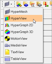
1.	On the Client Selector toolbar, select HyperView.The HyperView environment displays.

hm-4350-29

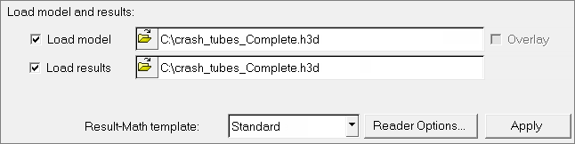
2.	In the panel area, load the model and results files.

Note:

Load *.h3d files for both the model and result files.

hm-4350-30

3.	Click Apply.

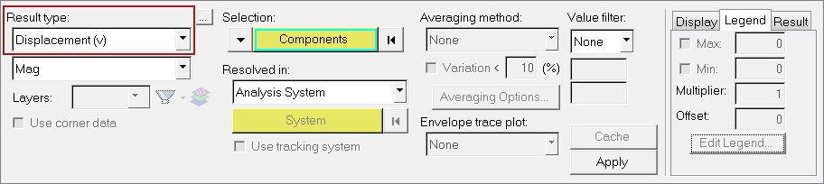
4.	On the Results toolbar, click to open the Contour panel.

5.	Review displacement (v) results by setting the Result type to Displacement (v).

hm-4330-33

6.	Click Apply.

hm-4350-33

7.	In the Results browser, review steps and increments.

hm-4350-32

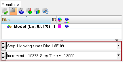
8.	On the Animation toolbar, set the animation mode to transient.

hm-4350-31

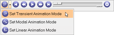
9.	Review the animation by clicking .

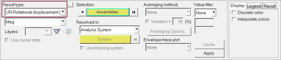
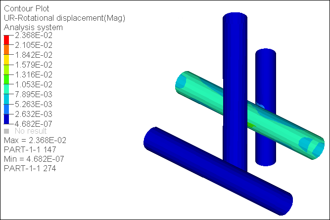
10.	Review UR-Rotational displacement (v) results by setting the Result type to UR-Rotational displacement (v) in the Contour panel.

hm-4330-38

11.	Click Apply.

hm-4350-34

HM-4350: Pre-Processing for Crashing Tubes Analysis using Abaqus

HM-4350: Pre-Processing for Crashing Tubes Analysis using Abaqus

HM-4350: Pre-Processing for Crashing Tubes Analysis using Abaqus

Model Files

Exercise

Defining the Abaqus *ORIENTATION in HyperMesh

Local directions for this model

Understanding boundary conditions for this model

Method 1:

Method 2:

X

Y

Notes:

See Also: