Study on Trajectories

---

Overview

---

Two balls are now considered in order to study the behavior of impacting spherical balls.

The balls’ behavior is described using the parameters (angles and velocities) shown in Fig 11. The numerical results are compared with the analytical solution, assuming a perfect elastic rebound (coefficient of restitution is equal to 1).

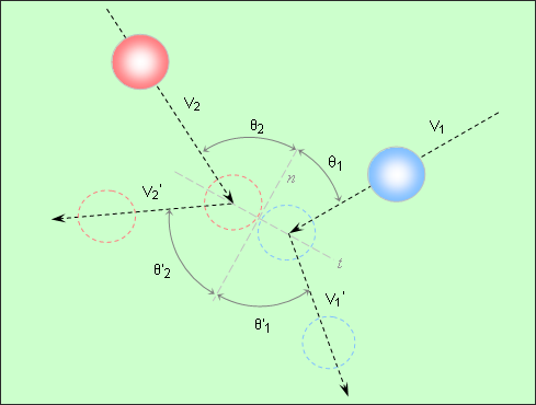
Fig 11: Problem data.

Initial values: V1 = 0.7m.s-1; V2 = 1m.s-1; 1 = 40°; 2 = 30; massball = 44.514g.

Modeling Methodology

The balls and the table have the same properties, previously defined for a pool game. The dimensions of the table are 900 mm x 450 mm x 25 mm and the balls’ diameter is 50.8 mm. The balls and the table are meshed with 16-node thick shell elements for using the type 16 Lagrangian interface.

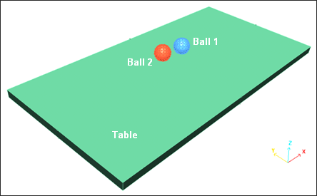
Fig 12: Mesh of the problem (16-node thick shells).

The initial translational velocities are applied to the balls in the /INIV Engine option. Velocities are projected on the X and Y axes.

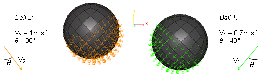
Fig 13: Initial velocities applied on the balls (initial position).

Gravity is considered for the balls (0.00981 mm.ms-2 ).

The ball/ball and balls/table contact is modeled using the type 16 interface (slave nodes/master 16-node thick shells contact). The interface defining the ball/ball contact is shown in Fig 14.

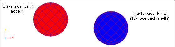
Fig 14: Master and slave sides for the type 16 Lagrangian interface.

Analytical Solution

Take two balls, 1 and 2 from masses m1 and m2, moving in the same plane and approaching each other on a collision course using velocities V1 and V2, as shown in Fig 15.

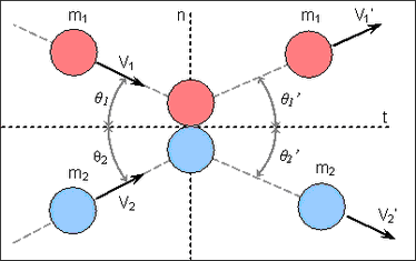
Fig 15: General problem of collision between two balls.

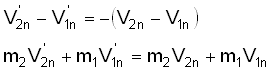
Velocities are projected onto the local axes n and t. To obtain the velocities and their direction after impact, the momentum conservation law is recorded for the two balls:

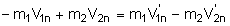
or

The shock is presumed elastic and without friction. Maintaining the translational kinetic energy is respected as there is no rotational energy:

Such equality implies that the recovering capacity of the two balls corresponds to their tendency to deform.

This condition equals one of the elastic impacts, with no energy loss. Maintaining the system’s energy gives:

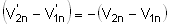
This relation means that the normal component of the relative velocity changes into its opposite during the elastic shock (coefficient of restitution value e is equal to the unit).

The following equations must be checked for normal components:

The equations system using V’1 and V’2 as unknowns is easily solved:

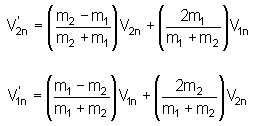
It should be noted that these relations depend upon the masses ratio.

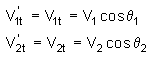
As the balls do not suffer from velocity change in the t-direction, maintaining the tangential component of each sphere’s velocity provides:

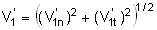
The norms of velocities after shock result from the following relations.

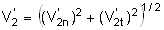
In this example, balls have the same mass: m1 = m2.

Therefore:

and

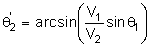
The norms of the velocities are given using the following relations, depending on the initial velocities and angles. Used to determine the analytical solutions (angles and velocities after collision):

 

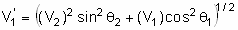
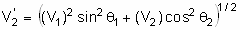
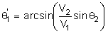
By recording the projection of the velocities, directions after shock can be evaluated using relation. Used to determine the analytical solutions (angles and velocities after collision):

 

 

Simulation Results: Comparison of Numerical Results with the Analytical Solution

---

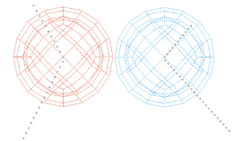
The following diagram shows the trajectories of the balls’ center point obtained using numerical simulation before and after collision.

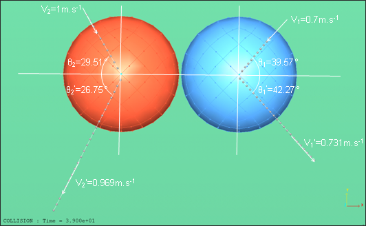
Fig 16: Trajectories of balls (center of gravity).

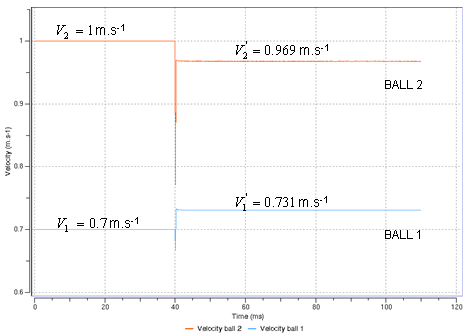
Fig 17: Variation of velocities (collision at 40 ms).

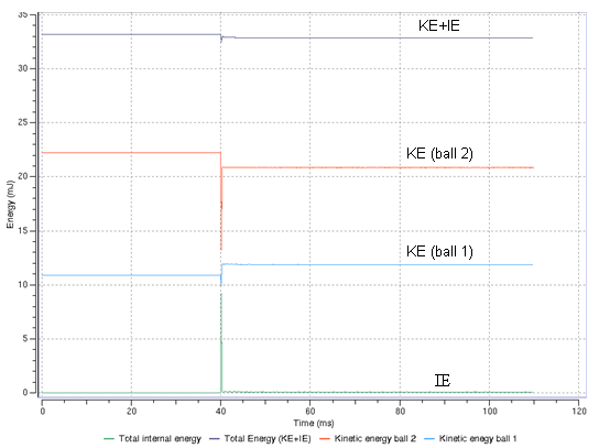
Fig 18: Energy assessment.

For given initial values of V1, V2, 1 and 2, simulation results are reported in Table 1.

Table 1: Comparison of results for after collision

Conclusion

---

The simulation corroborates with the analytical solution. The 16-node thick shells are fully-integrated elements without hourglass energy. This modeling provides a good transmission of momentum. However, the type 16 interface does not take into account the quadratic surface on the slave side (ball 2), due to the node to thick shell contact. Accurate results are obtained for a collision without penetrating the quadratic surface of the slave side in order to confirm impact between the spherical bodies.

A fine mesh could improve the results.