Control: Differential Equation

Model Element

Description

Control_Diff defines a single, first order, user-defined differential equation in MotionSolve. A single, dynamic state is associated with the differential equation. This state is integrated along with the rest of the system states. The differential equation may be a function of the user-defined dynamic state and any other instantaneous state of the system that can be accessed using MotionSolve expressions.

The Control_Diff model element is available in two types. The first, probably the most convenient, is of type expression and the second is of type user-subroutine.

The governing differential equation may be either explicit or implicit.

Format

<Control_Diff

id = "integer"

label = “Name of Control_Diff element”

is_implicit = { "TRUE" | "FALSE" }

ic = "real"

[ ic_dot = "real" ]

[ is_static_hold = { "TRUE" | "FALSE" } ]

{

type = "EXPRESSION"

expr = "motionsolve_expression"

| type = "USERSUB"

usrsub_dll_name = "valid_path_name"

usrsub_param_string = "USER( [[par_1][, ...][, par_n]] )"

usrsub_fnc_name = "custom_fnc_name" >

| type = "USERSUB"

script_name = "valid_path_name"

interpreter = "PYTHON" | "MATLAB"

usrsub_param_string = "USER( [[par_1 [, ...][,par_n]] )"

usrsub_fnc_name = "custom_fnc_name" >

}

Attributes

Element identification number (integer>0). This number is unique among all Control_Diff elements.

label

The name of the Control_Diff element.

is_implicit

A Boolean that specifies whether the derivative of the state is implicitly defined by the differential equation or not.

"TRUE" implies that the derivative is implicitly defined. "FALSE" implies that the derivative is explicitly defined.

If not specified, is_implicit defaults to FALSE

See Comment 3 for a more detailed explanation on the difference between explicit and implicit differential equations.

is_static_hold

A Boolean that specifies whether the value of the dynamic state is kept fixed or not during static equilibrium and quasi static solutions.

"TRUE" implies that the value of the dynamic state is kept constant during static and quasistatic solutions.

"FALSE" implies that the value of the dynamic state is allowed to change during static equilibrium or quasistatic solutions.

See Comment 7 for more information on how this is accomplished.

If not specified, is_static_hold defaults to FALSE.

Defines the initial condition for the dynamic state. This parameter is required. If not specified, ic defaults to 0.0.

ic_dot

Defines the initial condition for the time derivative of the dynamic state. This is required only when the differential equation is implicitly defined.

See Comment 3 for the distinction between explicit and implicit differential equations.

If not specified, ic_dot defaults to 0.0

type

Select from EXPRESSION and USERSUB. Specifies how the Control_Diff is defined. The EXPRESSION option specifies that the differential equation is defined as a MotionSolve expression that can be evaluated at run-time. The USERSUB option indicates that the differential equation is specified in a user-written subroutine. The parameters "usrsub_param_string" and
"usrsub_dll_name" are used to provide more information about the user defined subroutine.

expr

Defines an expression that defines the differential equation. Use this parameter only when type = EXPRESSION. Any valid run-time MotionSolve expression can be provided as input.

usrsub_param_string

The list of parameters that are passed from the data file to the user defined DIFSUB. Use this keyword only when type = USERSUB is selected.

usrsub_dll_name

Specifies the path and name of the DLL or shared library containing the user subroutine. MotionSolve uses this information to load the user subroutine specified by usersub_fnc_name in the DLL at run time. Use this keyword only when type = USERSUB is selected.

usrsub_fnc_name

Specifies an alternative name for the user subroutine DIFSUB.

script_name

Specifies the path and name of the user written script that contains the routine specified by usrsub_fnc_name.

interpreter

Specifies the interpreted language that the user script is written in. Valid choices are MATLAB or PYTHON.

Comments

Control_Diff is quite versatile and has many different applications in modeling multi-body systems. User defined dynamic states are commonly used to create low pass filters, apply time lags to signals, model simple feedback loops and integrate signals. The signal may be used to define forces, used as independent variables for interpolating through splines or curves, used as input signals for generic control modeling elements, or used to define program output signals.

The MotionSolve expressions and user-subroutines allow you to define fairly complex user defined dynamic states.

The expression type is used when the algorithm defining the differential equation is simple enough to be expressed as a simple formula. In many situations, the dynamic state is governed by substantial logic and data manipulation. In such cases, it is preferable to use a programming language to define the value of a Control_Diff. A user defined subroutine, allows you to accomplish this. For more information on defining a user subroutine for the Control_Diff model element, please refer to the DIFSUB documentation.

3.	Ordinary differential equations may be explicit or implicit.

An explicit differential equation has the form:

; y is the variable being defined, u are state dependent inputs (obtained from the rest of the system) and t is the independent variable.

Here is an example of an explicit, 2nd order differential equation:

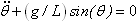
(no state dependent input u)

You may recognize it as the equation of motion for a simple pendulum.

An implicit differential equation has the form:

; y is the variable being defined, u are state dependent inputs (obtained from the rest of the system) and t is the independent variable.

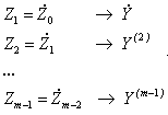
Here is an example of an implicit, 1st order differential equation:

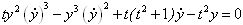
(no state dependent input u)

This equation cannot be symbolically transformed to define explicitly. For implicit differential equations, an initial guess for is also required.

The key differences between the two representations are summarized below:

•	In the explicit case, the derivative of the dynamic state is explicitly defined. The expression defines the derivative of the user defined state .

•	In the implicit case, the derivative has to be solved for. The expression defines the residue of the differential equation, .

•	An important requirement for implicitly defined ordinary differential equations is that the partial derivative, , must always be non-zero. This is satisfied for explicit differential equations if they were expressed in an implicit manner.

4.	To define implicit differential equations, you need to access both the value of the dynamic state associated with a CONTROL_DIFF and its time derivative.

•	The function DIF(ID) allows you to access the value of the dynamic state.

•	The function DIF1(ID) allows you to access the time derivative of the dynamic state.

5.	The equation defining the time derivative of the dynamic state (explicitly or implicitly) should be smooth for efficient solution. Lack of smoothness may be inadvertently introduced into the equations the following ways.

•	By experimental data (sampled as Splines). The data may have a lot of noise.

•	Logic in a user subroutine or a function expression that may introduce kinks or even discontinuities in the function if not careful.

6.	If you wish to introduce a set of differential equations into the model, use the Control_StateEqn modeling element to accomplish this. Unlike Control_Diff, Control_StateEqn can handle arrays of differential equations.

7.	The behavior of the dynamic state associated with a Control_Diff object during static and quasistatic solutions is governed by the attribute, is_static_hold.

is_static_hold = "TRUE"

If the solution is done at time t=0, the state is kept fixed at the value specified by ic. If the solution is being done after a dynamic analysis, then the value is kept fixed at the last value obtained from a dynamic simulation. The equation defining the Control_Diff is replaced with the following equation:

, where y* is a constant.

Note that when the value of the dynamic state is kept fixed, the time derivative no longer is zero, since the inputs u changes. This may lead to transients in the solution, if a dynamic solution were to be subsequently performed.

is_static_hold = "FALSE"

The state is not kept constant, but is allowed to change as the state of the entire system changes during the solution process. Here is how this is accomplished:

•	For static and quasi-static solutions, the derivative of the dynamic state is set to zero. This converts the Control_Diff to an algebraic equation for these two analyses.

Explicit differential equations become:

Implicit differential equations become:

During the equilibrium solution, the inputs u change, as the system changes its configuration to meet the equilibrium conditions. The above equations are solved to compute y for a given value of u.

This mechanism ensures that the time derivative of the dynamic state is zero at the end of the static or quasi-static solution, and ensures a smooth subsequent dynamic analysis.

Example

This example demonstrates how a higher order differential equation may be converted into a set of coupled first order differential equations and then modeled using Control_Diff elements.

The image below shows a simple mass, spring-damper system. The mass is constrained to move in one direction. The mass of the system is 0.5 Kg, the stiffness of the spring is 104 N/m, and the damping in the system is 102 Ns/m. CD_ExFig

Let x denote the spring deformation. The governing equation for this simple system is:

The order of a differential equation is the highest derivative that it contains. For instance, a first-order differential equation contains only first derivatives.

The governing equation for the system in the image above is therefore a second order differential equation. In order to convert it to the first order form, introduce a velocity variable vx. The velocity is defined as the time derivative of the displacement.

The governing equation can now be written as two first order differential equations.

Assume the system starts with the initial conditions x=0.2m, and vx = 0.0. The two differential equations may now be specified as follows.

The differential equation defining vx (note: C/M=2*1e2, K/M=2*1e4):

<Control_Diff

id = "1"

label = “SolverDiff name”

is_static_hold = "FALSE"

ic = "0.0"

type = "EXPRESSION"

expr = "-200*DIF(1) – 20000*DIF(2)">

The differential equation defining x:

<Control_Diff

id = "2"

label = “SolverDiff name”

is_static_hold = "FALSE"

ic = "0.2"

type = "EXPRESSION"

expr = "DIF(1)">

A few points to note:

•	The function DIF(ID) refers to the state defined by Control_Diff, ID="id".

•	The velocity state is defined by Control_Diff, ID="1". Therefore the velocity state is accessed using DIF(1).

•	The displacement state is defined by Control_Diff, ID="2". Therefore the displacement state is accessed using DIF(2).

•	Control_Diff, ID="1" and Control_Diff, ID="2" are coupled differential equations. For example, the first equation refers to the state of the second, and vice-versa.

•	Forward referencing of user-defined states is allowed. For example, the first differential equation may refer to the user defined state in the second differential, even though the second equation has not yet been defined.

The use of additional states to reduce the order of the system is quite common. The reduction method shown above can be generalized to deal with higher order systems.

Assume that a system is characterized by the math order differential equation shown below.

For the sake of notational convenience, let

Introduce m-1 new variables Zi, defined as follows:

CD_ExFig6

The original math order equation can now be replaced by m first order differential equations of the form:

CD_ExFig7

Model Element
Description
DIFF defines a single, first order, user-defined differential equation in MotionSolve. For additional information on the definition of DIFF, please see Control_Diff.
Declaration
def DIFF(id, LABEL="", IC=[], STATIC_HOLD=False, FUNCTION="", IMPLICIT=False, ROUTINE="", INTERPRETER="", SCRIPT=""):
Attributes
id	Element identification number (integer>0). This number is unique among all DIFF elements.
LABEL	The name of the DIFF element.
IC	Specify the list of two values. The first value defines the initial condition for the dynamic state. This parameter is required. If not specified, it defaults to 0.0. The second value defines the initial condition for the time derivative of the dynamic state. This is required only when the differential equation is implicitly defined. If not specified, it defaults to 0.0.
STATIC HOLD	A Boolean that specifies whether the value of the dynamic state is kept fixed or not during static equilibrium and quasi-static solutions. "TRUE" implies that the value of the dynamic state is kept constant during static and quasi-static solutions. "FALSE" implies that the value of the dynamic state is allowed to change during static equilibrium or quasi-static solutions. If not specified, it defaults to FALSE.
FUNCTION	Defines an expression that defines the differential equation. Any valid run-time MotionSolve expression can be provided as input. Or The list of parameters that are passed from the data file to the user-defined PFOSUB.
IMPLICIT	A Boolean that specifies whether the derivative of the state is implicitly defined by the differential equation or not. "TRUE" implies that the derivative is implicitly defined. "FALSE" implies that the derivative is explicitly defined. If not specified, IMPLICIT defaults to FALSE.
ROUTINE	Specifies an alternative name for the user subroutine DIFSUB.
INTERPRETER	Specifies the interpreted language that the user script is written in. Valid choices are MATLAB or PYTHON.
SCRIPT	Specifies the path and name of the user written script that contains the routine.
Comments See Control_Diff
Example The examples below show how a DIFF element may be defined. DIFF(1, LABEL="SolverDiff Name", IC=[0,0], STATIC_HOLD=False, FUNCTION="-200DIF(1) – 20000DIF(2)" DIFF(2, LABEL="SolverDiff Name", IC=[.2,0], STATIC_HOLD=False, FUNCTION="DIF(1)" )

Control: Differential Equation

Control: Differential Equation

Control: Differential Equation

Model Element

Description

Format

Attributes

If not specified, is_implicit defaults to FALSE

Comments

Example

Model Element

Description

Declaration

Attributes

Comments

See Control_Diff

Example

See Also: