Model Element

Description

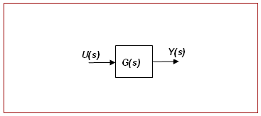
Control_SISO is an abstract modeling element that defines a linear, time invariant dynamic system in the Laplace domain. SISO stands for Single Input Single Output.  Such a dynamic system is characterized by a transfer function.  In practice, the transfer function is often characterized by experiments followed by curve fitting.  Modeling applications of this element include actuators (electrical, hydraulic, and pneumatic), vibration isolators (bushings and shock absorbers), and controllers (PID).

You specify the Control_SISO element by specifying the coefficients of the numerator and denominator polynomials that define the transfer function, along with one input (u) variable and one output (y) variable.  This is shown in the block diagram in the image below.

Block diagram representation of the Control_SISO element

U(s) and Y(s) represent the Laplace transforms of the time domain input and output variables and G(s) represents the transfer function given by:

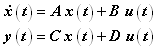
m and n denote the order of the numerator and denominator polynomials and must satisfy m ≤ n.

MotionSolve internally converts this Laplace domain element into the following time domain system of first order differential equations:

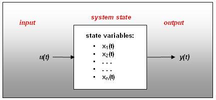
x is the state vector, u is the input variable, and y is the output variable. A, B, C, and D denote the state matrix, the input matrix, the output matrix, and the direct feed-through matrix, respectively.  The initial conditions for x are assumed to be zero.  The equations above are said to be in the state space form and are depicted schematically in the image below.

Input, Output, and States for a dynamic system

Format

<Control_SISO

      id                     = "integer"

    [ label                  = "string" ]

      x_array_id             = "integer"

      y_array_id             = "integer"

      u_array_id             = "integer"

    [ is_static_hold         = { "TRUE" |  "FALSE" } ]

      num_numerator_coef     = "integer"

      numerator_coef         = "real [ real real  …  real ] "

      num_denominator_coef   = "integer"

      denominator_coef       = "real [ real real …  real ] "

/>

Attributes

id

Element identification number (integer>0).  This number is unique among all Control_SISO elements.

label

The name of the Control_SISO element.

x_array_id

Specifies the ID of the Reference_Array used to store the states x of this Control_SISO. You can use the ARYVAL() function with this ID to access the states in a MotionSolve expression.  You can also use this ID in SYSFNC and SYSARY to access the state values from a user subroutine.

y_array_id

Specifies the ID of the Reference_Array used to store the output, y, of this Control_SISO. You can use the ARYVAL() function with this ID to access the states in a MotionSolve expression.  You can also use this ID in SYSFNC and SYSARY to access the output values from a user subroutine.

u_array_id

Specifies the ID of the Reference_Array used to store the input u of this Control_SISO. You can use the ARYVAL() function with this ID to access the states in a MotionSolve expression.  You can also use this ID in SYSFNC and SYSARY to access the input values from a user subroutine.

is_static_hold

Element identification number (integer>0).  This number is unique among all Control_SISO elements.

num_numerator_coef

An integer that specifies the number of coefficients in the numerator of the Control_SISO. num_state > 0.

numerator_coef

Specifies the coefficients, in the ascending powers of "s", of the numerator polynomial of the transfer function.

num_denominator_coef

An integer that specifies the number of coefficients in the denominator of the Control_SISO.
num_numerator_coef ≤ num_denominator_coef.

denominator_coef

Specifies the coefficients, in the ascending powers of "s", of the denominator polynomial of the transfer function.

Comments

Some examples of subsystems that could be "integrated" into a system model in MotionSolve include:

is_static_hold = "TRUE"

If the solution is done at time T = 0, the states are kept fixed at the value specified by the IC array.  If the solution is being done after a dynamic analysis, then the value is kept fixed at the last value obtained from a dynamic simulation. The equations defining the states for the Control_SISO are replaced with the following:

x(t*) = x*, where x* is a constant.

Note that when the dynamic states are kept fixed, their time derivatives no longer are zero at the end of the static equilibrium or a quasi-static step.  The inputs u will have changed.  This may lead to transients in the solution if a dynamic solution were to be subsequently performed.

is_static_hold = "FALSE"

The states are not kept constant, but allowed to change as the configuration of the entire system changes during the solution process. Here is how this is accomplished:

For static and quasi-static solutions, the derivative of the dynamic states is set to zero.  This converts the Control_SISO to a set of algebraic equations for these two analyses.

The differential equations become:

During the equilibrium solution, the input u changes as the system changes its configuration to meet the equilibrium conditions.  The above equations are solved to compute x for the current value of u.

This method ensures that the time derivative of the dynamic states is zero at the end of the static or quasi-static solution and ensures a smooth subsequent dynamic analysis.

Example

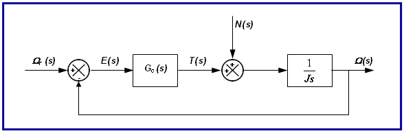
Consider the problem of maintaining a reference speed of a rotor in the presence of disturbance loads.  A block diagram of the control system is shown in the image below.

Block diagram for a rotor speed control system

•	denotes the reference speed.

•	denotes the actual speed.

•	denotes the controller transfer function.

One solution is to design a proportional integral (PI) controller (Ogata, 1995) with transfer function given by:

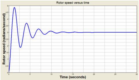
K and Kp denote the controller gains.  This controller can be modeled using the Control_SISO as follows:

<Control_SISO

    id                   = "303001"

    label                = “ControlSISO name”

    x_array_id           = "30300200"

    y_solver_id          = "30300300"

    u_solver_id          = "30300100"

    is_static_hold       = "FALSE"

    num_numerator_coef   = "2"

    numerator_coef       = "10. 1."

    num_denominator_coef = "2"

    denominator_coef     = "0. 1."

 />

This example is described in detail in the tutorial "Simulating a Single Input Single Output (SISO) Control System using MotionView and MotionSolve".  The image below, taken from the tutorial, shows the plot of a rotor speed versus time.

Plot of rotor speed versus time

Model Element

Description

TFSISO is an abstract modeling element that defines a linear, time invariant dynamic system in the Laplace domain. SISO stands for Single Input Single Output.  Such a dynamic system is characterized by a transfer function.  In practice, the transfer function is often characterized by experiments followed by curve fitting.  Modeling applications of this element include actuators (electrical, hydraulic, and pneumatic), vibration isolators (bushings and shock absorbers), and controllers (PID).

You specify the TFSISO element by specifying the coefficients of the numerator and denominator polynomials that define the transfer function, along with one input (u) variable and one output (y) variable.  This is shown in the block diagram in the image below.

Block diagram representation of the TFSISO element

U(s) and Y(s) represent the Laplace transforms of the time domain input and output variables and G(s) represents the transfer function given by:

m and n denote the order of the numerator and denominator polynomials and must satisfy m ≤ n.

MotionSolve internally converts this Laplace domain element into the following time domain system of first order differential equations:

x is the state vector, u is the input variable, and y is the output variable.  A, B, C, and D denote the state matrix, the input matrix, the output matrix, and the direct feed-through matrix, respectively.  The initial conditions for x are assumed to be zero.  The equations above are said to be in the state space form and are depicted schematically in the image below.

Input, Output, and States for a dynamic system

Declaration

def TFSISO(id, LABEL="", X=0, U=0, Y=0, STATIC_HOLD=False, NUMERATOR=[], DENOMINATOR=[]):

Attributes

id

Element identification number (integer>0).  This number is unique among all TFSISO elements.

LABEL

The name of the TFSISO element.

X

Specifies the ID of the ARRAY used to store the states x of this TFSISO. You can use the ARYVAL() function with this ID to access the states in a MotionSolve expression.  You can also use this ID in SYSFNC and SYSARY to access the state values from a user subroutine.

U

Specifies the ID of the ARRAY used to store the input u of this TFSISO. You can use the ARYVAL() function with this ID to access the states in a MotionSolve expression.  You can also use this ID in SYSFNC and SYSARY to access the input values from a user subroutine.

Y

Specifies the ID of the ARRAY used to store the output, y, of this TFSISO.  You can use the ARYVAL() function with this ID to access the states in a MotionSolve expression.  You can also use this ID in SYSFNC and SYSARY to access the output values from a user subroutine.

STATIC HOLD

A Boolean that specifies whether the value of the dynamic state is kept fixed or not during static equilibrium and quasi static solutions.

"TRUE" implies that the value of the dynamic state is kept constant during static and quasi-static solutions.

"FALSE" implies that the value of the dynamic state is allowed to change during static equilibrium or quasi-static solutions.

If not specified it defaults to FALSE.

NUMERATOR

Specifies the list of coefficients, in the ascending powers of "s", of the numerator polynomial of the transfer function.

DENOMINATOR

Specifies the list of coefficients, in the ascending powers of "s", of the denominator polynomial of the transfer function.

Comments

See Control_SISO

Example

The examples below show how a DIFF element may be defined.

TFSISO(303001, LABEL="ControlSISO Name",  X=30300200, U=30300100,  Y=30300300,  STATIC_HOLD=False, NUMERATOR=[10,1], DENOMINATOR=[0,1] )