Model Element
|
Description
|
Control_StateEqn is an abstract modeling element that defines a generic dynamic system. The dynamic system is characterized by a vector of inputs u, a vector of dynamic states x, and a vector of outputs y. The state vector x is defined through a set of differential equations. The output vector y is defined by a set of algebraic equations. The image below illustrates the basic concept of a dynamic system.
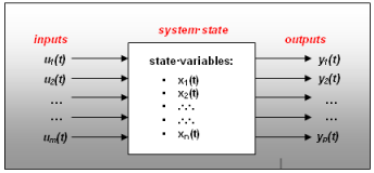
Inputs, Outputs, and States for a dynamic system.
Two types of Control_StateEqn elements are available in MotionSolve.
| 1. | Linear Dynamical Systems: These are characterized by four matrices: A, B, C, and D. These are related to the dynamical system in the following way: |
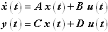
The four matrices A, B, C, D are all constant valued. The first equation defines the states. The second equation defines the outputs.
The A matrix is called the state matrix. It defines the characteristics of the system. If there are "n" states, then the A matrix has dimensions n x n. Either A or B or A+B are required to be non-singular.
The B matrix is called the input matrix. It defines how the inputs affect the states. If there are "m" inputs, the size the B matrix is n x m.
The C matrix is called the output matrix. It defines how the states affect the outputs. If there are "p" outputs, the size the C matrix is p x n.
The D matrix is called the direct feed-through matrix. It defines how the inputs directly affect the outputs. The size the D matrix is p x m..
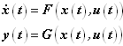
| 2. | Nonlinear Dynamical Systems: These are characterized by two vector functions: F() and G(). These are related to the dynamical system in the following way: |

The function F() returns the time derivative of x, when it is provided x(t) and u(t). The function G() returns the outputs y, when it is provided x(t) and u(t). Both F() and G() are required to be defined in user defined subroutines.
|
Format
|
<Control_StateEqn
id = "integer"
[ label = "string" ]
x_array_id = "integer"
ic_array_id = { "integer" | "0" }
[ is_static_hold = { "TRUE" | "FALSE" } ]
[ y_array_id = "integer" ]
[ u_array_id = "integer" ]
{
type = "LINEAR"
a_matrix_id = "integer"
[ b_matrix_id = "integer" ]
[ c_matrix_id = "integer" ]
[ d_matrix_id = "integer" ]
| type = "USERSUB"
num_state = "integer"
num_output = "integer"
usrsub_param_string = "USER( [[par_1][, ...][, par_n]] )"
usrsub_dll_name = "valid_path_name"
[ usrsub_fnc_name = "custom_fnc_name" ]
[ usrsub_der1_name = "custom_fnc_name" ]
[ usrsub_der2_name = "custom_fnc_name" ]
[ usrsub_der3_name = "custom_fnc_name" ]
[ usrsub_der4_name = "custom_fnc_name" ]
| type = "USERSUB"
num_state = "integer"
num_output = "integer"
script_name = valid_path_name
interpreter = "PYTHON" | "MATLAB"
usrsub_param_string = "USER( [[par_1 [, ...][,par_n]] )"
[ usrsub_fnc_name = "custom_fnc_name" ]
[ usrsub_der1_name = "custom_fnc_name" ]
[ usrsub_der2_name = "custom_fnc_name" ]
[ usrsub_der3_name = "custom_fnc_name" ]
[ usrsub_der4_name = "custom_fnc_name" ]
>
}
</Control_StateEqn>
|
Attributes
|
id
|
Element identification number (integer>0). This is a number that is unique among all Control_StateEqn elements.
|
label
|
The name of the Control_StateEqn element.
|
is_static_hold
|
A Boolean that specifies whether the values of the dynamic states, x, are kept fixed during static equilibrium and quasi-static solutions.
"TRUE" implies that the dynamic states are kept constant during static and quasistatic solutions.
"FALSE" implies that the dynamic state are allowed to change during static equilibrium or quasistatic solutions.
See Comment 5 for more information on how this is accomplished.
|
x_array_id
|
Specifies the ID of the REFERENCE_ARRAY used to store the states "x" of this Control_StateEqn. You can use the ARRAY() function with this ID to access the states in a MotionSolve expression. You can also use this ID in SYSFNC and SYSARY to access the state values from a user subroutine.
|
y_array_id
|
Specifies the ID of the REFERENCE_ARRAY used to store the outputs "y" of this CONTROL_STATEEQN. You can use the ARRAY() function with this ID to access the states in a MotionSolve expression. You can also use this ID in SYSFNC and SYSARY to access the output values from a user subroutine.
|
u_array_id
|
Specifies the ID of the REFERENCE_ARRAY used to store the inputs u of this Control_StateEqn. You can use the ARRAY() function with this ID to access the states in a MotionSolve expression. You can also use this ID in SYSFNC and SYSARY to access the input values from a user subroutine.
|
ic_array_id
|
Specifies the ID of the Reference_Array used to store the initial values of the states, x of this Control_StateEqn. You can use the ARYVAL() function with this id to access the states in a MotionSolve expression. You can also use this ID in SYSFNC and SYSARY to access the initial state values from a user subroutine.
|
type
|
Specifies the type of dynamic system being modeled. Select one from the choices "LINEAR" or "USERSUB". "LINEAR" specifies that the dynamic system being modeled is linear. The system definition is achieved by specifying the IDs of the A, B, C, and D matrices. "USERSUB" specifies that the dynamic system being modeled is defined in user defined subroutines. The dynamic system can be linear or nonlinear.
See Comments 2 and 3 for more information about this.
|
a_matrix_id
|
Specifies the ID of the Reference_Matrix object containing the state matrix for a linear Control_StateEqn. The A matrix encapsulates the intrinsic properties of the dynamic system. For instance, the eigenvalues of A represent the eigenvalues of the system. Similarly, the eigenvectors of A represent the mode shapes of the dynamic system. A is a constant valued matrix. It is required to be invertible. If there are n states, the A matrix is of dimension n x n. Use only when type = "LINEAR".
|
b_matrix_id
|
Specifies the id of the Reference_Matrix object containing the input matrix for a linear Control_StateEqn. The B matrix determines the contribution of the inputs u to the state equations.
B is a constant valued matrix. If there are m inputs and n states, the B matrix is of dimension n x m.
Use only when type = "LINEAR".
|
c_matrix_id
|
Specifies the id of the Reference_Matrix object containing the output matrix for a linear Control_StateEqn. The C matrix determines the contribution of the states x to the outputs y. C is a constant valued matrix. If there are p outputs and n states, the C matrix is of dimension n x p.
Use only when type = "LINEAR".
|
d_matrix_id
|
Specifies the id of the Reference_Matrix object containing the feed-thru matrix for a linear Control_StateEqn. The D matrix determines the contribution of the inputs u to the outputs y. D is a constant valued matrix. If there are p outputs and m inputs, the D matrix is of dimension p x m.
Use only when type = "LINEAR".
|
num_state
|
An integer that specifies the number of states in the Control_StateEqn. num_state > 0.
Use only when type = "USERSUB".
|
num_output
|
An integer that specifies the number of outputs in the Control_StateEqn. num_output > 0.
Use only when type = "USERSUB".
|
usrsub_param_string
|
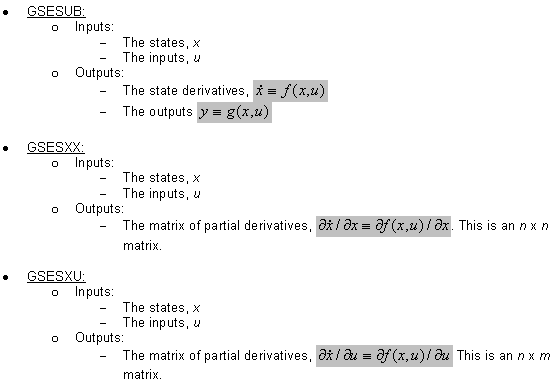
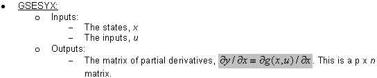
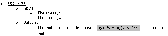
The list of parameters that are passed from the data file to the user defined subroutines GSESUB, GSEXX, GSEXU, GSEYX and GSEYU. See Comment 4 for more explanation about these user defined subroutines. Use only when type = "USERSUB". This attribute is common to all types of user subroutines and scripts.
|
usrsub_dll_name
|
Specifies the path and name of the DLL or shared library containing the user subroutine. MotionSolve uses this information to load the user subroutines GSESUB, GSEXX, GSEXU, GSEYX and GSEYU in the DLL at run time. Use only when type = "USERSUB".
|
usrsub_fnc_name
|
Specifies an alternative name for the user subroutine GSESUB.
|
usrsub_der1_name
|
Specifies an alternative name for the user subroutine GSEXX.
|
usrsub_der2_name
|
Specifies an alternative name for the user subroutine GSEXU.
|
usrsub_der3_name
|
Specifies an alternative name for the user subroutine GSEYX.
|
usrsub_der4_name
|
Specifies an alternative name for the user subroutine GSEYU.
|
script_name
|
Specifies the path and name of the user written script that contains the routine specified by usrsub_fnc_name.
|
interpreter
|
Specifies the interpreted language that the user script is written in. Valid choices are MATLAB or PYTHON.
|
Comments
|
| 1. | Control_StateEqn element is quite versatile and has many different applications in modeling multi-disciplinary systems. This element may be used to embed complex externally-defined subsystems within a MotionSolve system model. The external subroutines may be hand-written or they may just be an interface to a complete 3rd party application. |
Some examples of 3rd party applications that could be "integrated" into a system model in MotionSolve include:
| • | Control, Hydraulic and other generic system representations, generated by Real Time Workshop, a product from The MathWorks, Inc., that can generate C code corresponding to a Simulink block diagram. |
| • | Sophisticated tire models that include their own internal states. |
| • | Nonlinear finite element packages that define small to medium sized nonlinear finite element component in the MotionSolve model. |
| • | Automotive driver models that mimic human driving behavior in car models. |
| • | Frequency and amplitude dependent bushings that contain their own internal states. |
| 2. | The "LINEAR" version of a Control_StateEqn may be represented as a block diagram as shown in the image below. |
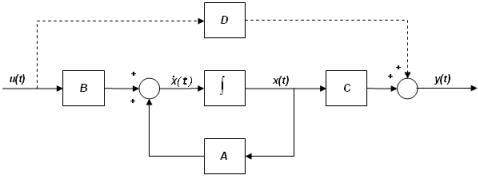
A block diagram representation of linear Control_StateEqn
| 3. | The "USERSUB" version of a Control_StateEqn may also be represented as a block diagram as shown in the image below. |
A block diagram view of a nonlinear, continuous Control_StateEqn.
| 4. | The "USERSUB" version of a Control_StateEqn is more complex than most modeling elements that are defined via user defined subroutines. |
Five user subroutines may be needed. The first, GSESUB is required. The other four, GSEXX, GSEXU, GSEYX, GSEYU, are required only when a stiff integrator (VSTIFF or MSTIFF) is used.
| 5. | The behavior of the dynamic states associated with a Control_StateEqn element during static and quasistatic solutions is governed by the attribute is_static_hold. |
is_static_hold = "TRUE"
If the solution is done at time T=0, the states are kept fixed at the value specified by the IC array. If the solution is done following a dynamic simulation, then the value is kept fixed at the last value obtained from the dynamic simulation. The equations defining the states for the Control_StateEqn are replaced with the following:
x(t*) = x*, where x* is a constant.
Note that when the dynamic states are kept fixed, their time derivatives are no longer zero at the end of the static equilibrium or a quasi-static step because the inputs u, which are typically time dependent, have changed. This may lead to transients if a dynamic solution were to be subsequently performed.
is_static_hold = "FALSE"
The states are not kept constant, but allowed to change as the configuration of the entire system changes during the solution process. Here is how this is accomplished.
For static and quasi-static solutions, the derivative of the dynamic states is set to zero. This converts the Control_StateEqn to a set of algebraic equations.
The differential equations become:

During the equilibrium solution, the inputs u change as the system changes its configuration to satisfy the equilibrium conditions. The above equations are solved to compute x for the current value of u.
This method ensures that the time derivative of the dynamic states is zero at the end of the static or quasi-static solution, and thus avoids introducing transients in a subsequent dynamic simulation.
|
Example
|
Friction is often modeled as a dynamic system. This example demonstrates the implementation of the LuGre (Lundt-Grenoble) friction model that incorporates both stiction and dynamic friction. The model has inputs, outputs, and states and can thus be implemented as a Control_StateEqn.
Friction is modeled as a set of "bristles" that represent micro-welds between two contacting surfaces. When a tangential force is applied at the contact patch, the bristles deflect like springs. Bristle stiffness and damping generate the friction forces. If the deflection is sufficiently large, the bristles start to slip. The model includes the Stribeck effect, which takes into account the dependency of the frictional force on velocity. The model also includes rate dependent friction phenomena such as varying break-away force and frictional lag. The LuGre model has the form:
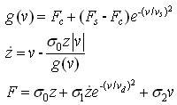
z denotes the bristle deflection.
 are stiction and dynamic friction coefficients. are stiction and dynamic friction coefficients.  is instantaneous value of the normal force. is instantaneous value of the normal force.
This dynamical system model for friction has the following properties:
| • | One input (m=1): The current slip velocity, v. |
| • | One state (n=1): The "bristle" deflection, z. |
| • | One output(p=1): The friction force, F. |
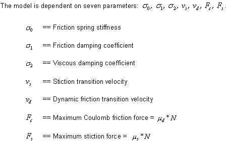
| • | Seven design parameters: 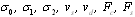 . . |
The friction model is applied to the simple system shown in the image below.
A test rig for the LuGre Friction model
The model depicts a one dimensional problem. Movement is only allowed in the global X direction. The system consists of two masses, Body 1 and Body 2 that are connected by a spring of stiffness K = 2 N/m. The mass of each body is 1 Kg. The bodies rest in the XY global plane. A motion of 0.1*time is applied in the global x-direction at the CM of body 2. The center of mass of body 1 is denoted by marker 666. The coordinate x defines the x-displacement of Body 1. It is measured by the MotionSolve expression DX(666). The sliding velocity of Body 1 is measured by the expression VX(666).
The system works as follows:
| • | Body 1 is originally at rest. |
| • | Due to the motion input at Body 2, the spring is stretched. The spring force increases. |
| • | The friction force, F, counteracts the spring force, and there is a small bristle deformation. |
| • | When the spring force reaches the break-away force, Body 1 starts to slide. |
| • | The friction force now decreases rapidly due to the Stribeck effect. The spring contracts, and the spring force decreases. |
| • | The mass slows down and the friction force increases because of the Stribeck effect and the motion stops. |
| • | The phenomenon then repeats. |
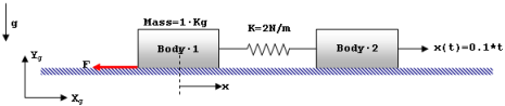
The design parameters for the model are:
For this example, the Control_StateEqn element is:
< Control_StateEqn
id = "1"
is_static_hold = "FALSE"
x_solver_array_id = "101"
y_solver_array_id = "102"
u_solver_array_id = "103"
ic_solver_array_id = "104"
type = "USERSUB"
num_state = "1"
num_output = "1"
usrsub_param_string = "USER(666, 1E5, 316.23, 0.4, 1E-3, 2E-3, 1, 1.5)"
usrsub_dll_name = "/staff/olaf/work/Lugre/Lugre.so">
</Control_StateEqn>
The X and Y arrays are defined as:
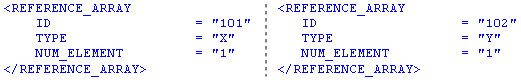
The U and IC arrays are defined as:
The Reference_Variable that provides the input to the friction model is defined as:
<Reference_Variable
Id = "1"
Type = "Expression"
Expr = "Vx(666)">
</Reference_Variable>
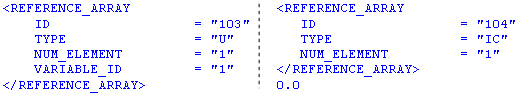
The time history of the velocity of Body 1 and the frictional force acting on it is shown in the plots below:
The response of the LuGre model.
|