Flexible Body Generation

The following information is common to all flexible body generation methods and details the initial partitioning step involved.

Dynamic Reduction is used to reduce a finite element model of an elastic body to the interface degrees of freedom and a set of normal modes for inclusion as a flexible body in a multi-body dynamics analysis.

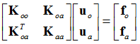
For the purpose of deriving the reduced matrices, the displacement vector u may be partitioned into displacements of inner, u0 and outer, ua interface/attachment degrees of freedom.

(1)

Here, the subscript o denotes the inner degrees of freedom, and the a denotes the interface degrees of freedom (for example, ASET entry).

The interface nodes that are used in the component mode synthesis process for the construction of mode shapes should be coincidental to the set of force-bearing nodes in the subsequent multi-body dynamics analysis. In a multi-body dynamics model, the flexible body interacts with other components of the model through joints, constraints, or force elements, which are connected or applied on the nodes of the flexible body. Except for body forces due to gravity or acceleration of the flexible body, all nodes that are subject to constraint or applied forces in the multi-body dynamics analysis are denoted as force-bearing nodes.

The purpose of specifying the interface nodes for CMS is mainly to account for the static deformation due to constraints or applied forces acting on the interface nodes. A huge number of eigenmodes is required if these static modes are omitted. The flexible deformations due to constraint forces, compared to the deformation due to the body inertia forces, are often dominant in most constrained models; therefore, the inclusion of all force-bearing nodes as interface nodes is an essential step to get accurate results from subsequent flexible multi-body dynamics analysis.

The static equilibrium is given as:

(2)

Where, K is the stiffness matrix and f is the force vector with the corresponding subscripts depicting the partitioning based on the inner/interface degrees of freedom.

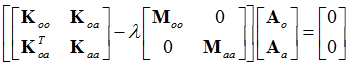
The eigenvalue problem for a normal modes analysis of the body using a diagonal mass matrix, M is illustrated as:

(3)

Where, A are the partitioned eigenvectors of the system. Only eigenvectors pertaining to the non-attachment degrees of freedom, Aa, are used in the subsequent generation of the combined modal matrix (see CBN and GM methods below).

The goal of the flexbody generation is to find a set of orthogonal modes Aort that represent the displacements u of the reduced structure such that:

Where, q is the matrix of modal participation factors or modal coordinates which are to be determined by the analysis.

The Craig-Bampton and Craig-Chang methods of Dynamic Reduction are available.

Craig-Bampton Method

Normal modes analysis of the fixed-interface system yields the diagonal matrix of eigenvalues, and the matrix of eigenmodes, . In the normal mode analysis, you can select the cut-off frequency or the number of modes to be solved. This determines the column dimension of .

In addition, a static analysis is performed to generate the static modes. With constrained interface degrees of freedom, a unit displacement in each interface degree of freedom is applied while all other interface degrees of freedom are fixed. With unconstrained (freed) interface degrees of freedom, the inertia relief will be performed by applying a unit force in each interface degree of freedom. This yields the static displacement modes/matrix As and the interface forces, fa .

Reduced modal stiffness, Kreduced , and mass, Mreduced , matrices are now generated as follows:

The displacement matrix is written as:

Which yields,

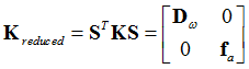
An orthogonalization step that transforms S into a set of orthogonal modes Aort is now performed. See Eigenvector Orthonormalization below for more information.

Craig-Chang Method

This method uses a system that is unconstrained (free-free) and therefore has six rigid body modes. Normal modes analysis of the system yields the diagonal matrix of eigenvalue, and the matrix of eigenmodes, . In the normal mode analysis, you can select the cut-off frequency or the number of modes to be solved. This determines the column dimension of . The eigenmodes AR associated with the rigid body modes will be normalized with respect to the mass matrix such that:

An equilibrated load matrix fe is formed as follows:

As seen in previous sections, fa is the force vector at the attachment points. In Craig-Chang method, the attachment point forces is a collection of force vectors which have otherwise all zero entries except a unit force along each degree of freedom of the interface nodes. The equilibrated load matrix fe is applied in an inertia relief static analysis to remove the rigid body modes. The equilibrated load matrix is applied, as follows:

The resulting modes As are called the inertia relief attachment modes.

Reduced modal stiffness and mass matrices are now generated using the displacement matrix (combines static modes and eigenmodes):

The reduced matrices are calculated as,

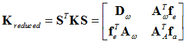
An orthogonalization step that transforms S into a set of orthogonal modes Aort is now performed. See Eigenvector Orthonormalization below for more information.

Eigenvector Orthonormalization

First, a new eigenvalue problem using the reduced matrices in the previous two sections is solved as shown below:

The resulting eigenvectors Anew are used to transform the original shapes/displacement vectors S into the set of orthogonal modes, Aort.

It can be shown that the resulting modes are orthogonal with respect to the system/original stiffness matrix K and mass matrix, M.

Note that the Orthogonal modes Aort are normalized with respect to the mass matrix M, therefore the final reduced matrices appear as:

The orthonormalized modes are input to other multi-body dynamics solvers (like MotionSolve), as modal representations of the flexible body in the subsequent analysis.

Loading on Flexible Body

If loading is applied to the flexible body in OptiStruct, then it will be reduced out as modal distributed loads and provided as an input to MotionSolve. The conversion is performed as follows:

In MotionSolve, any arbitrary displacement field of the flexible body is approximated by:

Where, q is the m by 1 modal participation vector.

Suppose fi is the ith distributed load defined in the FE model (f is an n by 1 vector, where n is the number of nodes on which the load is applied), ui is the corresponding displacement field, and u is any arbitrary displacement field of the flexible body, as mentioned above. The virtual work due to fi is:

Taking variation on both sides of the arbitrary displacement field equation, you have,

Substituting for u:

Now define the modal distributed load, as:

Each modal distributed load is a m by 1 vector.

The above modal distributed loads, along with their load ID in the FE model, should be pre-computed in OptiStruct and written as new modal distributed load blocks in the .h3d file. In addition, the corresponding displacement fields ui should enter the mode shapes S in the CMS process.

Input and Output

Flexible body generation is activated by the presence of the I/O Option CMSMETH. The I/O Option references a CMSMETH bulk data entry which defines the method (only CC and CB methods apply to flexible body generation), frequency range or number of modes to be calculated. Only one subcase is allowed per model. The interface degrees of freedom are defined using ASET or ASET1 bulk data statements. An MPC reference is allowed. While subcases are irrelevant for this run mode, if the model has multiple subcases, the MPC reference must match for all subcases. Subcase information entries other than MPC are ignored.

In general, offsets should not be used in flexible body generation. However, PARAM, CMSOFST may be used to allow small offsets for shell elements.

The orthogonal modes Aort and the corresponding eigenvalues are exported to a flexh3d file by default. The modal stresses and strains can be output optionally using the STRESS and STRAIN output statements. Sets can be applied to reduce the amount of data. The export of the model to this file can be controlled using the MODEL output statement.

Recovering MBD Analysis results in OptiStruct

After MotionSolve is run, it is possible to recover displacements, velocities, accelerations, stresses, and strains for the flexbody in OptiStruct in order to create .op2 and .h3d results files for fatigue analysis. The procedure is explained below.

After running MotionSolve, a residual run can be made to recover displacement, velocity, acceleration, stress, and strain results for interior grids and elements in the Flex Body based on the modal participation results from MotionSolve. After running MotionSolve, a resulting <filename>.mrf file is created that contains MotionSolve results including the modal participation factors at each time step for the Flex Body for transient analysis. In the residual run, the Flex Body <filename>_recov.h3d file and the .mrf results file are specified using the ASSIGN data:

ASSIGN,H3DMBD,30101,’pfbody_1_recov.h3d'

ASSIGN,H3DMBD,30102,’pfbody_2_recov.h3d'

ASSIGN,MBDINP,10,’pfbody.mrf'

Where, the 10 in the ASSIGN,MBDINP data references the SUBCASE for which the MotionSolve results will be used. In SUBCASE 10, instead of performing a transient analysis, OptiStruct will just use the results from MotionSolve.

The 30101 and 30102 in the ASSIGN,H3DMBD data refer to the Flex Body ID’s in the .mrf file.

For transient analysis, the number of time steps in the transient analysis run must match the number of time steps used in the MotionSolve analysis. While the transient analysis data is ignored, there must still be some dummy loading data (TLOAD, DAREA, and TABLED data). A sample of input data for a transient analysis run is shown below:

OUTPUT OP2

OUTPUT H3D

ASSIGN,H3DMBD,30103,MBD_pfbody_BODY_2_PROP_6_recov.h3d

ASSIGN,H3DMBD,30102,MBD_pfbody_BODY_1_PROP_9_recov.h3d

ASSIGN,H3DMBD,30104,MBD_pfbody_BODY_3_PROP_10_recov.h3d

ASSIGN,MBDINP,1,MBD_pfbody_mbd.mrf

SUBCASE 1

TSTEP(TIME) = 4

DLOAD = 3

DISPLACEMENT = ALL

STRESS = ALL

SPC = 1

BEGIN BULK

GRID 9999999 $ Dummy GRID since at least one GRID is required

$------+-------+-------+-------+-------+-------+-------+-------+-------

TSTEP 4 300 .0003333 1

TLOAD1 3 3 DISP 2

TABLED1 2 LINEAR LINEAR

+ 0.0 1.0 10.0 1.0ENDT

$ Dummy load on the dummy grid

SPC 1 9999999 1

SPCD 3 9999999 1 -200.0

ENDDATA

A dummy grid and a dummy load has been added for the OptiStruct analysis run.